Application of Advanced Statistical Process Control Methodologies to Regional Consumption Process Monitoring: Evidence from the West African Economic and Monetary Union (WAEMU) Bloc

Digitalization Inclusion and Development

Pioneers the application of statistical process control to regional economic phenomena. Using EHCVM household survey data (2018/2019 and 2021/2022) from WAEMU’s 103 administrative regions, a multivariate partially linear copula-based profile monitoring system (MPLPMS) tracks mean and variance-covariance of food and non-food consumption. Findings reveal persistent regional disparities in poverty and inequality post-pandemic, with policy implications aligned with UN SDGs 1, 10, and 17.

Author

Ibrahim Niankara

Published

10 April 2026

Working Paper · Brass Digital Lab · Abu Dhabi, UAE
Author: Ibrahim Niankara — Al Ain University, College of Business, Brass Digital Lab
Contact: Ibrahim.niankara@aau.ac.ae
Keywords: Household consumption; Poverty and inequality; Process monitoring; Statistical process control; Multivariate copula models; WAEMU
JEL Codes: C14 · D12 · I32 · O55 · R12 · Q56

Introduction

Process monitoring is the practice of leveraging advanced data analytics, statistical techniques, and real-time monitoring tools, to gain a deeper understanding of process behavior, and optimize performance parameters to achieve desired outcomes (Ghasemi et al., 2023). At its core, process monitoring entails the continuous observation, analysis, and evaluation of systems, activities, or operations to ensure their efficient functioning, identify deviations from expected performance, and facilitate timely corrective actions (Jalilibal et al., 2022). Process monitoring plays a crucial role in ensuring compliance with regulatory standards, meeting customer expectations, and enhancing organizational resilience in the face of disruptions or uncertainties (Sabahno & Amiri, 2023).

Due to its significance in not only enhancing operational efficiency, but also enabling organizations to adapt to changing environments, mitigate risks, and drive continuous improvement, process monitoring has received significant attention among academic scholars (Jalilibal et al., 2022). Consequently, process monitoring research has grown to occupy a pivotal role in both academic inquiry and practical application across various fields, ranging from manufacturing and supply chain management to service industries and beyond (Busababodhin & Amphanthong, 2016; Song et al., 2021; Xu et al., 2024).

In the realm of business and industry, process monitoring research has yielded invaluable insights into the intricacies of production processes, supply chain dynamics, and service delivery mechanisms (Easton et al., 2022; Haq & Ali, 2024). Beyond the realm of traditional business processes, the significance of process monitoring research extends theoretically to broader socio-economic contexts, including regional economic blocs. In these settings, process monitoring could offer a powerful framework for analyzing complex economic phenomena, such as household consumption patterns, trade dynamics, and policy effectiveness. By applying process monitoring principles to economic processes, researchers could uncover underlying trends, assess policy impacts, and inform evidence-based decision-making to drive sustainable development, poverty reduction, and inclusive growth within regional contexts.

Despite this great potential, previous studies on process monitoring have predominantly concentrated on business processes, particularly in manufacturing and non-manufacturing sectors (Ahmadi Yazdi et al., 2024; Jalilibal et al., 2022; Sabahno et al., 2020; Tasias & Nenes, 2012; Zaidi et al., 2023), overlooking the critical role and intricate dynamics of economic processes such as consumption, particularly within the context of regional economic blocs. However, characterized by economic integration and cooperation among member states, regional economic blocs represent unique environments where understanding consumption dynamics is crucial for fostering economic stability, promoting inclusive growth, and advancing sustainable development goals (Niankara, 2023).

Indeed, recent studies have evaluated household consumption patterns using classical methods such as Ordinary Least Squares (OLS), with Machine Learning approaches including Random Forest regression (E. Lee et al., 2024). In the context of the European Union (EU) for instance, using social expenditure, resilience and EU regional policy funding together with multi-level modeling, Ferraro et al. (2021) reported a reduction in social exclusion from EU funding, especially in Eastern European countries. Similarly, in the context of the Economic Community of the West African States (ECOWAS), using Dynamic Panel Data analysis with Generalized Methods of Moments (GMM) techniques to evaluate the influence of digital financial inclusion (DFI) on household consumption among 13 ECOWAS countries, Faton & Chabossou (2024) reported DFI to significantly enhance household consumption expenditure, which is positively mediated by economic growth. Recent evidence further underscores this nexus between financial inclusion (FI), digital inclusion, and multidimensional outcomes in developing economies. For instance, Naveenan et al. (2024) demonstrate that FI and DFI, moderated by digital inclusion, enhance health outcomes in emerging markets through entropy-weighted indices, suggesting potential synergies with consumption monitoring. Similarly, Wang et al. (2024) highlight DFI’s role in reducing household multidimensional poverty, influenced by financial environments such as credit availability, while Kamble et al. (2024) emphasize FI and digital financial literacy’s contributions to financial well-being, providing demand-side insights applicable to WAEMU’s regional disparities.

Despite the pivotal role of household consumption in driving economic activity and shaping societal well-being, a notable gap remains in the literature regarding the application of process monitoring methodologies to consumption processes, especially within regional economic blocs (García-Gómez et al., 2021). This oversight underscores the urgency of examining household consumption through the lens of process monitoring, given its significance in informing policy decisions.

Therefore, focusing on the West African Economic and Monetary Union (WAEMU), the current research seeks to address this literature gap, by applying statistical process monitoring and control methodologies to economic processes, particularly household consumption process at the regional economic bloc level. The unique socio-economic context and development priorities of WAEMU, offers a rich terrain for exploring household consumption dynamics and their implications for poverty, inequality, and sustainable development outcomes (Niankara, 2023). Comprising eight francophone West African countries, WAEMU stands at the intersection of diverse socio-economic dynamics, cultural influences, and development challenges (Thiombiano et al., 2022). Despite its economic cohesion and shared currency, disparities in living standards are still present (Yameogo & Omojolaibi, 2022), underscoring the importance of understanding and monitoring household food and non-food consumption patterns within the region. This holistic approach not only complements existing research in business process monitoring but also broadens the scope of inquiry to encompass a crucial aspect of economic activity often overlooked in traditional process monitoring frameworks. To this end, consistent with recently proposed schemes for the simultaneous monitoring of multivariate multiple linear profiles’ parameters (Haq & Ali, 2024; Rahimi et al., 2022; Sabahno & Amiri, 2023), this study is guided by the following objectives:

Develop a comprehensive methodological framework for simultaneously tracking the mean and variance-covariance parameters of household consumption processes within WAEMU.
Investigate drivers and determinants of household consumption behavior within the region, including socio-economic, demographic, Spatio-temporal, and digital financial inclusion factors (Kamble et al., 2024; as evidenced by Wang et al., 2024), analyzing their implications for poverty and inequality dynamics.
Translate insights from consumption process monitoring into actionable policy recommendations for WAEMU policymakers and stakeholders, facilitating the design of targeted interventions aligned with the United Nations SDGs.

Consistent with these objectives, the study seeks to answer the following research questions:

How can we develop a robust methodology for simultaneously tracking the mean and variance-covariance parameters of household consumption processes within the West African Economic and Monetary Union?
What are the key socio-economic, demographic, and Spatio-temporal drivers of household consumption behavior within WAEMU, and how do they contribute to poverty and inequality dynamics across member states?
How can insights from consumption process monitoring be leveraged to design targeted interventions and policies for poverty and inequality reduction within the WAEMU context, in alignment with the United Nations SDGs?

To address these questions, the paper is structured as follows: Section 2 describes the methodology, focusing on the data source, the proposed multivariate partially linear profile monitoring system (MPLPMS) for household consumption, along with its theoretical underpinnings. Section 3 presents the results; Section 4 discusses the findings; and finally, Section 5 concludes the analysis with future research suggestions.

Methodology

Considering the growing consensus in the value of using household economic surveys to assess household economic wellbeing (Nghiem et al., 2022; Russell et al., 2018; Yu et al., 2021), this paper draws from the relatively new research area of “profile monitoring” in statistical process monitoring (SPM) (Ahmadi Yazdi et al., 2024; Song et al., 2021; Yao et al., 2023), to extend for the first time the profile monitoring research field to include the economic process of household consumption. As a data driven methodology, the application of process monitoring to regional economy wide household consumption, requires access to the pertinent data. Therefore, this study uses the unique data source offered by the Enquête harmonisée sur les conditions de vie des ménages or “Harmonized Survey on Households Living Standards” (EHCVM), as described next.

The Data

Recently initiated by the WAEMU commission as a joint program with the World Bank, EHCVM is a nationally representative survey that aims to produce standardized household level data covering all country members of the West African Economic and Monetary Union (Programme d’Harmonisation et de Modernisation des Enquêtes sur les Conditions de Vie des ménages (PHMECV), 2023). The first edition of the survey was conducted in 2018/2019, with the second and latest edition conducted in 2021/2022. To account for consumption seasonality, each edition of the survey is typically implemented in two stages/waves within each country, by the respective National Statistical Institute, and covers households’ representative of the geopolitical zones at both, rural and urban level. The first stage sampling corresponds to the random selection of enumeration areas, while the second stage sampling corresponds to the selection of households within each enumeration area.

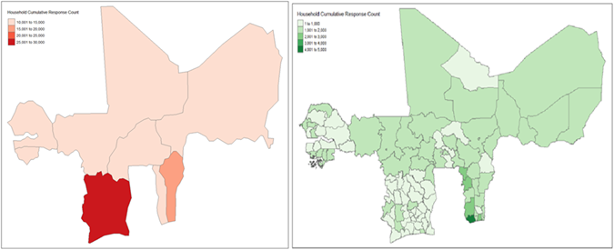
The first edition of the survey was carried out between October 2018 and July 2019 for the first wave; and between April 2019 and July 2019 for the second wave. However, the second edition took place between August and December 2021 (first wave), and between April and December 2022 (second wave). Each edition of the survey uses two main survey instruments (a household level questionnaire and a community level questionnaire) to produce nationally representative estimates for households’ annual consumption spending, and a range of demographic and socio-economic characteristics for the civilian non-institutionalized populations in each country member. Figure 1 describes the cross-national (left panel) and cross-regional (right panel), cumulative count, and geographical coverage of the survey data, while Table 1 summarizes the characteristics of the data collection (survey sampling) design.

Table 1: Study Data Sample Characteristics

Country	First Edition (Ed1)				Second Edition (Ed2)				Total raw Sample Size		Final Treated data Sample
	WAVE 1		WAVE 2		WAVE 1		WAVE 2				Final Sample Size (n)		Final Retention Rate (%)
	Oct. 2018 to Dec. 2018		Apr. 2019 to Jul. 2019		Aug. 2021 to Dec. 2021		Apr. 2022 to Jul. 2022				Final Sample Size (n)		Final Retention Rate (%)
	Urban	Rural	Urban	Rural	Urban	Rural	Urban	Rural	Ed1	Ed2	Ed1	Ed2	Ed1	Ed2
Ivory Coast	2,744	3,746	2,531	3,971	2,736	3,768	2,520	3,984	12,992	13,008	12,992	12,965	100%	99.67%
Benin	1,940	2,057	2,000	2,015	1,949	2,064	2,003	2,016	8,040	8,032	8,012	8,032	99.65%	100%
Burkina Faso	1,577	1,930	1,572	1,931	1,647	1,938	1,691	1,900	7,070	7,176	7,010	7,176	99.15%	100%
Guinea Bissau	1,015	1,649	975	1,712	1,008	1,692	1,020	1,680	5,351	5,400	5,351	5,351	100%	99.09%
Mali	1,338	1,570	1,414	2,280	1,352	1,479	1,380	1,932	6,603	6,143	6,602	6,143	99.98%	100%
Niger	715	2,268	862	2,179	1,178	2,125	1,335	1,984	6,024	6,622	6,024	6,622	100%	100%
Senegal	1,961	1,607	1,980	1,608	1,980	1,608	1,980	1,608	7,156	7,176	7,156	7,120	100%	99.22%
Togo	1,034	1,897	1,236	2,004	1,236	2,004	1,236	2,004	6,171	6,480	6,171	6,462	100%	99.72%
WAEMU									59,407	60,037	59,318	59,871	99.85%	99.72%

Note: Ed1 = First Edition (2018/2019); Ed2 = Second Edition (2021/2022). Columns show urban/rural household counts per wave. The Ed2 Second Edition Wave 2 urban/rural breakdown for Senegal’s second edition waves are identical as they were collected in the same enumeration areas.

Figure 1: National (left panel) and Regional (right panel) cumulative frequency counts of household respondents within WAEMU

The Concept of Profile and Regional Consumption Profile Monitoring

To link the use of the above data source, the study builds on the quality control literature, where the quality of a product or a process is often characterised by a functional relationship called a “profile” (Ahmadi Yazdi et al., 2024), between a response variable and a set of independent or explanatory variables. In this framework, each profile is essentially a data frame of n measurements of a response and explanatory variables (Yao et al., 2023), and “profile monitoring” deals then with capturing and tracking overtime the functional curves, using data collected at regular time intervals (Ghasemi et al., 2023). It involves the use of various statistical techniques to monitor the process, and quickly detect abnormal/irregular deviations from the normal profile pattern (Krupskii et al., 2020).

Within this context, the publicly released versions of the EHCVM surveys contain several data folders and files, including the folder covering household welfare. This file tracks the same variables, including households’ total expenditures on food and non-food consumption, together with poverty threshold indicators, spatial and temporal deflators, and other relevant household characteristics as described in Table 2. Consistent with Yao et al. (2023), the two editions of the EHCVM survey then provide two WAEMU level household consumption profiles, whose summary statistics are provided in Table 3.

Table 2: Study Variables Definition and Description

Variable	Label	Description
`dali`	Log food consumption per capita	Daily log per-capita food expenditure (CFA francs)
`dnal`	Log non-food consumption per capita	Daily log per-capita non-food expenditure (CFA francs)
`dtot`	Total nominal consumption	Sum of food and non-food expenditure
`pcexp`	Real per-capita consumption	Inflation- and size-adjusted consumption
`year`	Survey year	2018 or 2021
`vague`	Survey wave	Wave 1 or Wave 2
`Residency`	Urban/Rural	Household residential area
`country`	Country	WAEMU member state (8 levels)
`region_2`	Administrative region	One of 103 regions
`hgender2`	Head gender	Male/Female
`hage`	Head age	Age of household head (years)
`hmstat4`	Marital status	Never/Monogamous/Polygamous/Previously married
`hreligion2`	Religion	Muslim/Christian/Animist/None
`heduc2`	Education level	None/Primary/Secondary/Higher
`LiteracyStat`	Literacy status	Literate/Illiterate
`hdiploma2`	Diploma certification	None/Elementary/Middle/High school/University
`hhandig2`	Handicap status	No handicap/Handicap
`hSectEconAct`	Economic sector	Primary/Secondary/Commerce/Services
`hOccupStat7D3`	Weekly occupation status	Occupied/Unemployed/Inactive
`hOccupStat12M`	Annual occupation status	Active/Inactive
`hhsize`	Household size	Number of household members
`hhweight`	Survey weight	Household sampling weight

Source: Extracted from the EHCVM (Programme d’Harmonisation et de Modernisation des Enquêtes sur les Conditions de Vie des ménages (PHMECV), 2023).

Given that the study relies on a periodic survey monitoring process, drawn every 2 years from the target population of household respondents in each country member of the WAEMU, and considering the variation in the sample sizes, and control limits (i.e. poverty thresholds — as lower control limit, with no upper bound), the resulting household consumption process monitoring framework is conceptualized as a variable parameters (VP) scheme (Sabahno et al., 2020; Tasias & Nenes, 2012). Therefore, using the response variables of “food consumption spending” and “non-food consumption spending”, which together capture the “needs” and “wants” aspects of the household consumption process at the regional scale; this study seeks to simultaneously monitor the (mean and variance-covariance) parameters of household (food and non-food) consumption process within WAEMU, for poverty and inequality performance improvement, and administrative simplicity in line with the UN SDGs (Sabahno & Amiri, 2023). To this end, the paper considers two simultaneous monitoring schemes, in line with phase I and II of standard business profile monitoring (Ghasemi et al., 2023; Sabahno et al., 2020):

Univariate/unconditional monitoring scheme, based on geo-spatial mapping of the inequality indices of Atkinson and Gini; and the poverty indices of Watts, Sen, and Foster. Used as graphical control charts in the context of regional inequality and poverty monitoring.
Multivariate/conditional monitoring scheme, using semi-parametric multivariate copula regression (Easton et al., 2022; Song et al., 2021; Yan, 2023).

By expanding the profile monitoring research field to include regional household consumption process, adding features of economic profile monitoring never considered before in the literature, this study pioneers an important framework for adequately addressing “poverty” and “inequality” at the regional economic bloc level, in accordance with the UN SDGs (Liu et al., 2015; Mahendra, 2024).

Theoretical Underpinning of the Proposed Consumption Profile Monitoring Framework

The multivariate partially linear profile monitoring system (MPLPMS) proposed in this paper draws on an integrated approach, combining income distribution and inequality theories, Amartya Sen’s Capabilities Approach, and two analytical frameworks: Copula-based dependence models and poverty and inequality decomposition frameworks. Together, these generally accepted theoretical pillars, provide a robust foundation for understanding and addressing household consumption expenditures determinants and effects on poverty and inequality (K.-K. Lee, 2014).

For instance, income distribution and inequality theories such as those proposed by Kuznets (2019), Jenkins (2017), Cowell (2015), and Atkinson (1996), provide explanations for how income distribution and inequality evolve over time. By offering metrics such as Lorenz curves and Gini coefficients to evaluate inequality (Fellman, 2012; Gastwirth, 1972), they emphasize the role of structural and policy factors in shaping disparities in consumption. Additionally, focusing on the ability of individuals and households to achieve well-being beyond nominal income or consumption, Sen’s Capabilities Approach (Sen, 1993; Shorrocks, 1995) highlights poverty as a deprivation of capabilities rather than purely a lack of resources. As a result, nominal consumption expenditures can be studied as proxies for households’ capabilities to achieve adequate living standards, thereby encouraging the inclusion of regional and socio-demographic differences in the analysis (Robeyns, 2005). Moreover, by providing a decomposition of total inequality into within-group and between-group components, theoretical frameworks such as the Poverty and Inequality Decomposition Frameworks (Ogwang, 2022), also support the proposed MPLPMS framework. Indeed, using tools such as the Foster-Greer-Thorbecke (FGT) poverty indices (J. Foster et al., 2010; J. E. Foster, 1984), and Theil or Atkinson measures of inequality (Bigsten, 2024; Cowell, 2000), these frameworks disaggregate poverty and inequality to analyse their determinants and effects across regions or demographic groups, thereby easing targeted interventions for reducing disparities. Furthermore, Copula-based frameworks are increasingly being applied in poverty and inequality studies to capture interdependencies between multiple dimensions of household consumption such as food and non-food spending (García-Gómez et al., 2021; Nai Ruscone, 2024; Niankara, 2023).

Therefore, combining these theories and theoretical frameworks allows for a holistic and integrated approach that accounts in a novel and ever evolving fashion households’ consumption behaviour, income distribution dynamics, and the interdependence between expenditure categories. Indeed, this integration specifically underpins the proposed MPLPMS framework by: (i) defining the economic context, since income distribution and inequality theories provide the macroeconomic foundation, explaining how disparities in resources translate into consumption inequalities; (ii) capturing human well-being, as Sen’s Capabilities Approach ensures that the framework goes beyond nominal consumption measures to capture multidimensional aspects of poverty and inequality; (iii) offering policy insights, from decomposition frameworks that isolate key drivers of poverty and inequality, allowing for the design of region-specific and demographic-targeted interventions; (iv) finally ensuring statistical precision from the robust and flexible Copula-based dependence modelling of the complex relationships between food and non-food consumption, essential for accurate policy recommendations.

The Multivariate Partially Linear Copula-Based Profile Monitoring System (MPLPMS) for Regional Household Consumption

Consistent with Verdier (2013), Song et al. (2021), Easton et al. (2022), and Yan (2023), the MPLPMS framework for regional household consumption monitoring builds on the copula methods presented in Niankara (2022), Niankara (2023), and Niankara et al. (2023), which provide a simple and efficient way to model multiple responses in a regression setting. To this end, we let Y_1 denote household expenditure on food within the WAEMU region, while Y_2 denotes expenditure on non-food items. As continuous random variables, Y_1 and Y_2 reflect respectively household welfare in terms of food and non-food consumption. Their joint cumulative distribution is expressed as F(y_1, y_2 \mid \boldsymbol{x}), where \boldsymbol{x} are covariates of household consumption, as illustrated in Figure 2. The copula-based representation of this function is given by:

F(y_1, y_2 \mid \boldsymbol{x}) = C\bigl(F_1(y_1 \mid \boldsymbol{x}),\; F_2(y_2 \mid \boldsymbol{x});\; \theta\bigr) \tag{1}

Here, F_1(\cdot) and F_2(\cdot) represent the marginal cumulative distribution functions of Y_1 and Y_2, each ranging from 0 to 1. The function C(\cdot) is a copula, which uniquely binds the marginal distributions without depending on their specific forms, while \theta is the copula parameter that quantifies the dependence between the two marginal distributions (Sancetta & Satchell, 2004; Schmelzer, 2015; Sklar, 1973). Parametric density functions, denoted as f_1(\cdot;\boldsymbol{\psi}_1) and f_2(\cdot;\boldsymbol{\psi}_2) are used to define the marginal distributions for Y_1 and Y_2, with parameters \boldsymbol{\psi}_k = (\mu_k, \sigma^2_k) corresponding respectively to the location, scale, and shape parameters of these marginal distributions (Mayr et al., 2012; Stasinopoulos & Rigby, 2008). The number of coefficients defining \boldsymbol{\psi}_1 and \boldsymbol{\psi}_2 is contingent on the chosen copula function. Trivedi & Zimmer (2007) have established a relationship between the correlation coefficient (or dependence parameter) \theta and Kendall’s \tau, a common measure of association within the range [-1,1]. This study compares the performance of the Gaussian copula, defined as C(u_1,u_2;\theta) = \Phi_2(\Phi^{-1}(u_1), \Phi^{-1}(u_2);\theta) for \theta \in (-1,1); where Kendall’s \tau = \frac{2}{\pi}\arcsin(\theta) and the transformation \theta = \sin\!\left(\frac{\pi\tau}{2}\right), with five other copulas (Clayton, Joe, Frank, Ali-Mikhail-Haq, and Farlie-Gumbel-Morgenstern copulas) for sensitivity analysis (Smith, 2023).

Specification of the Predictor Function for the MPLPMS

The general form of the predictor function under the various copula models across all N households in the study is:

\eta_{k,i} = \beta_{k,0} + \sum_{j=1}^{J} f_{k,j}(x_{ij}), \quad i = 1,\ldots,N,\; k = 1, 2, \theta \tag{2}

Here, N is the number of responding households in the study, \beta_{k,0} is the intercept of the regression model, and \boldsymbol{x}_i is the i-th sub-vector of the full covariate vector, which includes the outlined fixed and random factors in the conceptual framework. The f_{k,j}(\cdot) functions model generic effects chosen according to the type of covariate(s). Each is linearly approximated by b_j basis functions B_{j,l}(\cdot) and regression coefficients \boldsymbol{\gamma}_{k,j}, such that:

f_{k,j}(\boldsymbol{x}_j) = \sum_{l=1}^{b_j} \gamma_{k,j,l}\, B_{j,l}(\boldsymbol{x}_j) = \mathbf{B}_j \boldsymbol{\gamma}_{k,j} \tag{3}

Equation (3) implies that the evaluation vector f_{k,j} can be expressed as \mathbf{B}_j \boldsymbol{\gamma}_{k,j} with \mathbf{B}_j \in \mathbb{R}^{N \times b_j} as design matrix; thus allowing the rewriting of the predictor function in equation (2) as:

\boldsymbol{\eta}_k = \mathbf{1}_N \beta_{k,0} + \sum_{j=1}^{J} \mathbf{B}_j \boldsymbol{\gamma}_{k,j} \tag{4}

With \mathbf{1}_N being an N-dimensional vector of ones. This is more compactly rewritten as \boldsymbol{\eta}_k = \mathbf{X}_k \boldsymbol{\gamma}_k, with \mathbf{X}_k = [\mathbf{1}_N, \mathbf{B}_1, \ldots, \mathbf{B}_J] and \boldsymbol{\gamma}_k = (\beta_{k,0}, \boldsymbol{\gamma}_{k,1}^{\top},\ldots,\boldsymbol{\gamma}_{k,J}^{\top})^{\top}. As formulated, the smooth functions may represent spatio-temporal linear, non-linear, and random effects (Wood et al., 2016). Additionally, each f_{k,j} is associated with a quadratic penalty that enforces specific properties, including smoothness on the f_{k,j} function. The smoothing parameter \lambda_{k,j} controls the balance between fit and smoothness, determining the shape of f_{k,j}. The overall penalty is defined as \boldsymbol{\gamma}_k^{\top} \mathbf{S}_{\boldsymbol{\lambda}_k} \boldsymbol{\gamma}_k, where \mathbf{S}_{\boldsymbol{\lambda}_k} = \sum_j \lambda_{k,j} \mathbf{S}_j, with the smooth functions mean-centered for identification (Wood, 2017).

For variables with linear parametric effects (e.g. year of data collection, wave of data collection, household residency status, household head’s gender, marital status, education level, diploma certification status, economic sector of activity, weekly and annual occupational status), equation (4) becomes \boldsymbol{\eta}_k = \mathbf{X}_{k,\text{lin}} \boldsymbol{\beta}_k, with the design matrix formed by stacking all covariate vectors \boldsymbol{x}_i into \mathbf{X}_{k,\text{lin}}. For continuous variables (e.g. household size, household head’s age), f_{k,j} is approximated by \mathbf{B}_j \boldsymbol{\gamma}_{k,j}, where \mathbf{B}_j are known spline bases (Wood, 2003). The representation of the smooth functions is achieved using the regression beta-spline approach (Aguilera & Aguilera-Morillo, 2013; Amir et al., 2024), with \mathbf{B}_j as design matrix and comprising the basis functions for describing f_{k,j} curves of varying complexity (Eilers & Marx, 1996).

To introduce the spatial effects into the copula-based monitoring framework, the 103 local administrative regions within the eight WAEMU member countries, are split into discrete contiguous geographic units, with spatial coordinates integrated using a Markov random field approach (Acar & Sundararaghavan, 2016; Perperoglou et al., 2019). This captures the influence of neighbouring households within the same administrative regions in the overall WAEMU regional bloc. In this context, equation (4) becomes \boldsymbol{\eta}_k = \mathbf{X}_{k} \boldsymbol{\gamma}_k + \mathbf{Z}_s \boldsymbol{u}_s, where s \in \{1,\ldots,8\} makes up the labels of the eight country members, while \boldsymbol{u}_s represents spatial effects, with R = 103 denoting the number of administrative regions. The design matrix \mathbf{Z}_s \in \{0,1\}^{N \times R} that links each responding household i to the corresponding spatial effect is defined for all i as:

Z_{s,ir} = \begin{cases} 1 & \text{if household } i \text{ resides in region } r \\ 0 & \text{otherwise} \end{cases} \tag{5}

The smoothing penalty is based on the neighbourhood structure, ensuring that households in adjacent administrative regions share similar effects. The diagonal matrix for the quadratic penalty can therefore be expressed as:

S_{s,rr'} = \begin{cases} -1 & \text{if regions } r \text{ and } r' \text{ are adjacent} \\ n_r & \text{if } r = r' \\ 0 & \text{otherwise} \end{cases} \tag{6}

With S_{s,rr'} = -1 indicating the adjacency of any two local administrative regions r and r', while n_r represents the number of neighbors for region r. The quadratic penalty that results corresponds to the stochastic interpretation that \boldsymbol{u}_s follows a Gaussian Markov random field (Lindgren et al., 2011).

Estimation Details of the MPLPMS

Considering the full parameter vector \boldsymbol{\delta} = (\boldsymbol{\gamma}_1^{\top}, \boldsymbol{\gamma}_2^{\top}, \boldsymbol{\gamma}_{\theta}^{\top})^{\top}, and following Vatter & Chavez-Demoulin (2015), the copula function in equation (1) is expressed as the penalized log-likelihood:

\ell_p(\boldsymbol{\delta}) = \sum_{i=1}^{N} \log c\bigl(F_1(y_{1i};\boldsymbol{\psi}_{1i}),\; F_2(y_{2i};\boldsymbol{\psi}_{2i});\; \theta_i\bigr) + \sum_{k} \log f_k(y_{ki};\boldsymbol{\psi}_{ki}) - \frac{1}{2}\boldsymbol{\delta}^{\top} \mathbf{S}_{\boldsymbol{\lambda}} \boldsymbol{\delta} \tag{7}

To maximize the above joint likelihood function, all model parameters are simultaneously identified using penalized maximum likelihood estimation (Vatter & Nagler, 2018). An adaptive quadrature approach is employed for the numerical approximation of the penalized likelihood, based on the trust region algorithm presented in Marra & Radice (2017). To avoid overfitting, all smoothing parameters are determined via restricted maximum likelihood estimation as follows:

\mathcal{V}(\boldsymbol{\lambda}) = -2\log L_{\text{REML}}(\boldsymbol{\lambda}) = \log|\mathbf{S}_{\boldsymbol{\lambda}}|^{+} - \log|\mathbf{H}(\hat{\boldsymbol{\delta}})|^{+} - 2\ell_p(\hat{\boldsymbol{\delta}}) \tag{9}

With \mathbf{H}(\hat{\boldsymbol{\delta}}) = -\nabla^2 \ell_p(\hat{\boldsymbol{\delta}}), and |\cdot|^{+} the pseudo-determinant, the analytical score and Hessian Matrix of \ell_p are given by:

\nabla_{\boldsymbol{\delta}} \ell_p = \mathbf{X}^{\top} \mathbf{s} - \mathbf{S}_{\boldsymbol{\lambda}} \boldsymbol{\delta}, \qquad \nabla^2_{\boldsymbol{\delta}} \ell_p = -\mathbf{X}^{\top} \mathbf{W} \mathbf{X} - \mathbf{S}_{\boldsymbol{\lambda}} \tag{10}

Similarly, we obtain the first order conditions with respect to \boldsymbol{\psi}_1 and \boldsymbol{\psi}_2, with

\frac{\partial \ell_p}{\partial \boldsymbol{\gamma}_k} = \mathbf{X}_k^{\top} \mathbf{s}_k - \mathbf{S}_{\boldsymbol{\lambda}_k} \boldsymbol{\gamma}_k = \mathbf{0}, \quad k = 1, 2, \theta \tag{11}

The open-source statistical software R version 4.4.1 (R Core Team, 2024), and the GJRM package version 0.2-6.7 (Marra & Radice, 2024) are used for all estimation purposes. The estimation process involves iteratively maximizing the penalized log-likelihood function, by incorporating constraints on the smoothing parameters to balance model fit and smoothness, thereby ensuring a robust representation of household food and non-food wellness across all 103 regions and 8 countries in the WAEMU.

As outlined above, the multivariate partially linear Copula-based profile monitoring system (MPLPMS) can be used to evaluate spatial and temporal drivers of household well-being, at the regional economic bloc level (Niankara, 2023). This approach incorporates both linear and non-linear effects, as well as spatial dependencies, thereby providing a comprehensive framework for analysing the factors influencing household annual expenditures on food and non-food items.

Algorithmic Calibration and Sensitivity Analysis of the MPLPMS Framework

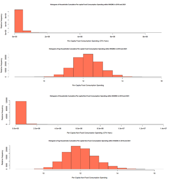
To identify the appropriate marginal distributions for the two outcomes, several candidates were considered. Given the typical right-skewness of consumption expenditure data, which are generally normalized through log transformation for regression modelling (see Figure 3), we considered among the marginal distribution candidates, the log-normal “LN”, for both food expenditure and non-food expenditure.

Figure 2: Normal Q-Q plots and Histograms of the normalized quantile residuals of log food consumption spending (top panel), and log non-food consumption spending (lower panel)

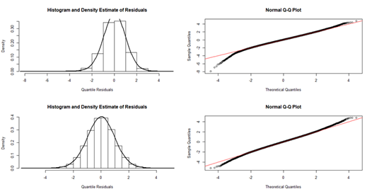
Figure 3: Histogram distribution of household per-capita food and non-food expenditure in levels and logged

The normal Q-Q plots of the normalized quantile residuals (Figure 2) suggest the log-normal (LN) distribution to be a good fit for both. Adopting the log-normal margins, the model was then fit under six different types of copula specifications for comparative model performance and sensitivity analysis (see Table 4). The estimation of the conditional mean, variance and covariance functions of the MPLPMS for regional household food and non-food consumption monitoring is done in R version 4.4.1, using the GJRM package, version 0.2-6.7 (Marra & Radice, 2024):

The specifications of the mean functions are given by eq.mu.1r and eq.mu.2r for the food and non-food consumption processes respectively. Similarly, the specifications of the variance functions are captured respectively by eq.sigma2.1r and eq.sigma2.2r for the food and non-food consumption processes, while the covariance function is given by eq.thetar. These are supplied to the estimating function gjrm() as a combined list flr. In the form of an optional argument, the estimating function also accommodates sampling weight hhweight that corrects for differing probability of household selection in the study sample. Finally, outr is the final R data object, containing the full outcome of the estimated model.

Model Sensitivity Analysis

To ensure robust statistical results and address potential model misspecification biases, the parameters of the MPLPMS are estimated under six different copula specifications, as shown in Table 4. The sensitivity analysis confirms satisfactory convergence diagnostics across all six specifications. This is evidenced by the largest absolute gradient values, the positive definiteness of the observed information matrix, and acceptable eigenvalue ranges from the implemented trust region iteration algorithm. Importantly, the estimated correlation coefficients display consistent signs and magnitudes across all models, reflecting robust parameter stability. Furthermore, the 95% confidence intervals for these coefficients do not contain zero, affirming their statistical significance and indicating meaningful interdependence between household food and non-food expenditures within WAEMU.

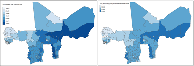
Among the models, the Gaussian Copula specification (M1) demonstrates the best performance, as it achieves the lowest Akaike Information Criterion (AIC) and Bayesian Information Criterion (BIC) values. These findings highlight its superior fit compared to the other copula specifications, leading to its selection for presenting the study’s results in Section 3. To further assess household vulnerability to poverty and inequality, Figure 4 presents the joint and independent cumulative probabilities that a given household spends below the WAEMU average consumption levels for food (dali) and non-food (dnal) items. The left panel assumes that food and non-food expenditures co-evolve over time and space, while the right panel assumes their independent evolution. The comparison of these two panels reveals spatially nuanced probability distributions, emphasizing the critical importance of controlling for the dependence structure between food and non-food consumption in the MPLPMS framework.

The sensitivity analysis underscores therefore the robustness of the MPLPMS framework in capturing the interdependence of consumption processes, offering valuable insights for addressing household poverty and inequality across WAEMU. By leveraging the Gaussian Copula specification, the analysis achieves a balanced approach that combines computational efficiency with reliable inference, ensuring its applicability to policy design within the region, and beyond.

Figure 4: Administrative regional level variations in predicted probabilities that a household spends jointly (left panel) and independently (right panel), below WAEMU level average on both food and non-food items consumption

Results

Study Sample (Household Consumption Profile) Descriptive Statistics

With summary statistics provided in Table 3, the two household consumption profiles extracted from the EHCVM (2018/2019 and 2021/2022) highlight important stylized facts. Indeed, a total of 59,318 households (29,048 in wave 1, and 30,270 in wave 2) responded fully to the survey in the first profile, while 59,871 households (29,642 in wave 1 and 30,229 in wave 2) participated in the second profile. At the spatial level, households are distributed unevenly across the 8 WAEMU states and 103 administrative regions.

Table 3: Summary Statistics of the Two Extracted Household Consumption Profiles from the EHCVM

Factor / Variable			2018/2019 Sample (N = 59,318)		2021/2022 Sample (N = 59,871)
Section	Variable	Units / Categories	Mean / Abs. Freq.	SD / % Rel. Freq.	Mean / Abs. Freq.	SD / % Rel. Freq.
Quantitative	`hhweight`	—	360.100	356.783	390.428	434.925
	`dali`	CFA franc	1,202,643	1,010,395	1,294,964	977,079
	`dnal`	CFA franc	1,141,136	1,569,584	1,202,660	1,207,233
	`dtot`	CFA franc	2,343,780	2,273,480	2,497,624	1,990,380
	`pcexp`	CFA franc	471,931	446,579.6	488,775	409,389.2
	`hhsize`	Persons	6.171	4.167	6.120	3.883
	`hage`	Years	45.63	14.66	47.87	14.39
Qualitative	`hgender`	Female	11,273	19.0%	12,196	20.4%
	`hgender`	Male	48,045	81.0%	47,675	79.6%
	`hmstat`	Never Married	5,931	10.0%	5,495	9.2%
		Monogamous	34,859	58.8%	34,744	58.0%
		Polygamous	11,106	18.7%	10,686	17.8%
		Previously Married	7,422	12.5%	8,946	14.9%
	`hreligion`	None	2,721	4.6%	2,150	3.6%
		Muslim	34,555	58.3%	35,158	58.7%
		Christian	16,850	28.4%	17,157	28.7%
		Animist	4,975	8.4%	5,219	8.7%
		Others	217	0.4%	187	0.3%
	`heduc`	None	35,658	60.1%	35,589	59.4%
		Primary	10,736	18.1%	10,258	17.1%
		Secondary	10,554	17.8%	11,576	19.3%
		Higher	2,370	4.0%	2,448	4.1%
	`hdiploma`	None	44,473	75.0%	44,434	74.2%
		At most elementary school certificate	1,234	2.1%	1,504	2.5%
		At most middle school certificate	4,562	7.7%	4,543	7.6%
		At most high school certificate	6,459	10.9%	6,807	11.4%
		At least university diploma	2,590	4.4%	2,583	4.3%
	`hhandig`	None	55,223	93.1%	56,034	93.6%
	`hhandig`	Major handicap	4,095	6.9%	3,837	6.4%
	`hSectEconAct`	Not Active	6,432	10.8%	7,666	12.8%
		Primary Sector	27,554	46.5%	27,006	45.1%
		Secondary Sector	6,158	10.4%	7,274	12.1%
		Tertiary Sector	12,398	20.9%	10,819	18.1%
		Commerce	6,776	11.4%	7,106	11.9%
	`hOccupStat7D`	Occupied	51,300	86.5%	51,171	85.5%
		Unemployed	931	1.6%	973	1.6%
		Inactive	7,087	11.9%	7,727	12.9%
	`hOccupStat12M`	Active	52,830	89.1%	53,042	88.6%
	`hOccupStat12M`	Not Active	6,488	10.9%	6,829	11.4%
	`vague`	Wave 1	29,048	49.0%	29,642	49.5%
	`vague`	Wave 2	30,270	51.0%	30,229	50.5%
	`Residency`	Rural	34,425	58.0%	33,715	56.3%
	`Residency`	Urban	24,893	42.0%	26,156	43.7%
	`region_2`	One of 103 regions	See cumulative frequency map in Figure 1
	`country`	One of 8 countries	See Ed1 column in Table 1		See Ed2 column in Table 1

Source: Author’s own, based on data extracted from the two editions of the EHCVM survey (Programme d’Harmonisation et de Modernisation des Enquêtes sur les Conditions de Vie des ménages (PHMECV), 2023).

Table 4: Performance Measures for the Six Specifications of the MPLPMS (Spatio-temporal Bivariate Copula Regression Models)

Model Specification	AIC	BIC	Trust Region Iteration Algorithm Characteristics			Trust Region Convergence Diagnostics			Estimated Dependence Parameters (95% C.I.)				n
Model Specification	AIC	BIC	Iterations before smoothing	Loops for smoothing	Iterations within loops	Largest \|gradient\|	Obs. info. positive definite	Eigenvalue range	σ²₁ (Food var.)	σ²₂ (Non-food var.)	ρ̂ (Copula par.)	τ̂ (Kendall's τ)	n
(M1) Gaussian	2,569,826,379	2,569,832,172	4	2	7	8.924×10⁻³	Yes	[85.465, 18,633,045,398]	0.512 (0.511, 0.513)	0.550 (0.549, 0.552)	0.517 (0.514, 0.520)	0.348 (0.346, 0.350)	119,189
(M2) Clayton	2,574,396,589	2,574,402,382	6	2	10	5.838×10⁻⁶	Yes	[98.502, 17,192,434,365]	0.521 (0.520, 0.523)	0.556 (0.555, 0.558)	0.697 (0.690, 0.705)	0.253 (0.251, 0.256)	119,189
(M3) Joe	2,573,820,991	2,573,826,784	6	2	11	4.636×10⁻⁶	Yes	[72.769, 16,528,850,103]	0.524 (0.523, 0.526)	0.566 (0.564, 0.567)	1.680 (1.670, 1.680)	0.269 (0.267, 0.271)	119,189
(M4) Frank	2,570,389,412	2,570,395,204	4	2	9	5.026×10⁻³	Yes	[83.181, 18,855,401,932]	0.518 (0.516, 0.519)	0.557 (0.555, 0.558)	3.760 (3.730, 3.790)	0.361 (0.359, 0.364)	119,189
(M5) Ali-Mikhail-Haq	2,572,488,599	2,572,494,392	6	2	11	5.288×10⁻⁶	Yes	[106.287, 16,485,500,353]	0.509 (0.508, 0.511)	0.548 (0.546, 0.549)	0.984 (0.891, 0.511)	0.277 (0.276, 0.278)	119,189
(M6) Farlie-Gumbel-Morgenstern	2,574,121,790	2,574,126,604	18	1	2	2.620×10⁻¹	Yes	[0.00992, 13,242,105,585]	0.504 (0.503, 0.505)	0.542 (0.540, 0.543)	1.000 (0.973, 1.000)	0.222 (0.216, 0.222)	119,189

Note: Numbers in parentheses are 95% Confidence Intervals (C.I.) on the respective parameters. σ²₁ = conditional variance of food consumption; σ²₂ = conditional variance of non-food consumption; ρ̂ = estimated copula dependence parameter; τ̂ = Kendall’s τ. Model M1 (Gaussian) achieves the lowest AIC and BIC, confirming best fit. Source: Author’s own, using data extracted from the two waves of the EHCVM survey (Programme d’Harmonisation et de Modernisation des Enquêtes sur les Conditions de Vie des ménages (PHMECV), 2023).

Regarding household characteristics, the average household size decreased slightly from 6.17 members in the first profile to 6.12 members in the second profile, with standard deviations of 4.17 and 3.88, respectively. Food consumption per household increased from an average of 1,202,643 CFA francs (SD: 1,010,395) in the first profile to 1,294,964 CFA francs (SD: 977,079) in the second profile. Similarly, non-food consumption increased from 1,141,136 CFA francs (SD: 1,569,584) to 1,202,660 CFA francs (SD: 1,207,233), reflecting an overall rise in household consumption over the survey periods. Moreover, the overall nominal consumption expenditures (dtot) of responding households, calculated as the sum of food (dali) and non-food (dnal) expenditures, increased between the two profiles. On average, households spent 2,343,780 CFA francs (SD: 2,273,480) in 2018/2019, which rose to 2,497,624 CFA francs (SD: 1,990,380) in 2021/2022. Similarly, the real per-capita personal consumption expenditure (pcexp), which adjusts household consumption for size and inflation, also increased slightly between the two profiles, from an average of 471,931 CFA francs (SD: 446,579.6) in 2018/2019 to 488,775 CFA francs (SD: 409,389.2) in 2021/2022, reflecting a modest improvement in individual household members’ economic well-being.

The demographic characteristics of household heads remained relatively stable. The majority were male, comprising 81% (48,045) in the first profile and 79.6% (47,675) in the second. The average age of household heads increased slightly, from 45.63 years (SD: 14.66) in the first profile to 47.87 years (SD: 14.39) in the second profile. Marital patterns showed a slight increase in the proportion of previously married household heads (from 12.5% to 14.9%), while the proportion of monogamous and polygamous heads slightly declined. In terms of religion, Muslims remained the majority, accounting for 58.3% (34,555) in the first profile and 58.7% (35,158) in the second profile, followed by Christians (28.4% and 28.7%, respectively) and animists (8.4% and 8.7%, respectively). The proportion of household heads reporting “no religion” declined slightly from 4.6% in the first profile to 3.6% in the second.

Socio-economic characteristics indicate that educational attainment improved marginally, with the proportion of household heads with secondary education increasing from 17.8% (10,554) to 19.3% (11,576). Similarly, those with higher education increased from 4% (2,370) to 4.1% (2,448). Conversely, household heads with primary education decreased by 1 percentage point from 18.1% (10,736) to 17.1% (10,258). Despite remaining the majority, the proportion of household heads reporting no educational attainment also decreased from 60.1% (35,658) in the first profile to 59.4% (35,589) in the second profile.

Physical health remained a key enabler for labor market participation, with 93.1% (55,223) and 93.6% (56,034) of household heads reporting no major handicap across the two profiles. Labor market participation patterns shifted slightly, with an increase in household heads reporting economic activity in the secondary sector, from 10.4% (6,158) to 12.1% (7,274), while those in the primary sector decreased from 46.5% (27,554) to 45.1% (27,006). Additionally, the occupation status of household heads over the past year shows stability in labor market participation, with active participation remaining high, decreasing marginally from 89.1% (52,830) in 2018/2019 to 88.6% (53,042) in 2021/2022.

Overall, the findings from the two household consumption profiles suggest consistent trends across WAEMU, with slight improvements in consumption levels, educational attainment, and labor market diversification between 2018/2019 and 2021/2022, reflecting gradual socio-economic progress within the region.

Findings from the Unconditional Monitoring Scheme

In addition to the above in-sample regularities, the findings from the unconditional monitoring scheme described below underscore critical variations in poverty and inequality between-and-within WAEMU countries, highlighting the urgency of both national and regional policy responses, through tailored and coordinated approaches, to achieve more balanced and inclusive economic growth. The unconditional monitoring of household consumption inequality within WAEMU is conducted at the national and sub-national/regional levels, using nominal indices of inequality, specifically the Atkinson and Gini indices. Similarly, the unconditional monitoring of household poverty within WAEMU is also conducted at the national and administrative regional levels, using the indices of Watts, Sen, and Foster (α = 0 and α = 1). These nominal indices are computed using tools and functions from the R library ineq (Zeileis, 2014), applied to household total nominal expenditures on food and non-food consumption for the fiscal years 2018 and 2021.

Regional Monitoring of Household Consumption Inequality within WAEMU

For the within-country regional monitoring of household welfare, we rely on the static and dynamic graphical control charts shown in Figures 5, 6, and 7 for regional inequality monitoring. Beginning with the Atkinson coefficient summarized in Figure 5, from the left panel that represents the data from the 2018 fiscal year, we observe a mean Atkinson coefficient of 0.1067, which suggests moderate inequality levels, with a range of 0.0595 to 0.1623 showing variability in inequality across the 103 regions. With the majority of regions clustered between 0.09 and 0.12, the distribution appears right skewed toward higher inequality.

From the right panel of Figure 5 that represents the Atkinson coefficients data for fiscal year 2021, we observe a mean Atkinson coefficient of 0.0888, suggesting a relatively lower inequality level than 2018. Although persistent regional disparities are still visible, the range of 0.0268 to 0.1595 indicates a broader reduction in inequality, with most regions clustered between 0.07 and 0.10, and fewer regions exhibiting extreme inequality.

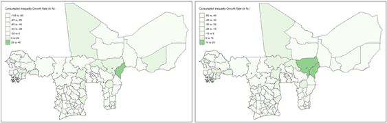
Overall, as characterised in the mostly negative regional growth rates shown in Figure 7, the observed decline in the average Atkinson coefficient suggests improvements in equality within the WAEMU region between 2018 and 2021. However, the increased standard deviation in 2021 (0.0229) compared to 2018 (0.0228) indicates a widening gap in inequality across regions. Similar patterns are observed with the Gini coefficient in Figures 6 and 7, supporting further the above described findings.

From a consumption process monitoring perspective, Figure 7 shows that while most regions have reduced household consumption inequalities between 2018 and 2021, recording negative growth rates for both the Atkinson and Gini coefficients, several regions still highlight increasing inequality levels. These include among others Dosso and Thillabery in Niger; the Sahel, Sud-Ouest and Boucle-du-Mouhoun regions in Burkina Faso; as well as Timbuktu and Mopti in Mali, just to name a few. These administrative regions warrant policy attention to ensure equity and sustainable poverty reduction across the WAEMU bloc.

Figure 5: Regional level distribution of household consumption inequality within WAEMU, based on the indices of Atkinson

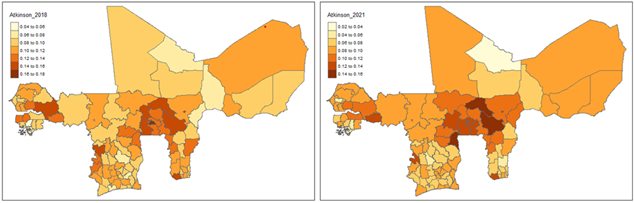
Figure 6: Regional level distribution of household consumption inequality within WAEMU, based on the indices of Gini

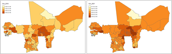
Figure 7: Regional level distribution of household consumption inequality growth rates between 2018 and 2021 within WAEMU, based on the indices of Atkinson (left panel) and Gini (right panel)

National Monitoring of Household Consumption Inequality within WAEMU

For the between-country national monitoring of household consumption inequality in WAEMU, we rely on the static and dynamic graphical control charts shown in Figures 8, 9, and 10. Starting with the Atkinson coefficient summarized in Figure 8, from the left panel representing the data for 2018, we note a cross-national average Atkinson coefficient of 0.1381, which suggests moderate inequality levels, with a range of 0.1066 (Guinea Bissau) to 0.1612 (Togo) indicating variability in inequality across the 8 national economies in WAEMU.

From the right panel of Figure 8, which showcases the cross-national Atkinson coefficients for 2021, we observe an average Atkinson coefficient of 0.1154, suggesting a relative reduction in household inequality, compared to 2018. The coefficients ranging from 0.0933 (Guinea Bissau) to 0.1346 (Burkina Faso) indicate a broader reduction in inequality.

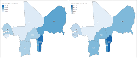
Overall, the negative national growth rates of the Atkinson coefficients characterized in Figure 10, suggest improvements in household consumption equality across WAEMU country members, between 2018 and 2021. Additionally, the decreased standard deviation in 2021 (0.0166) compared to 2018 (0.0227) indicates a narrowing gap in inequality across WAEMU nations.

To further assess the statistical significance of the observed cross-national means and variance fluctuations in the Atkinson and Gini coefficients, we rely on two formal ANOVA testing procedures. The results from the contemporaneous cumulative state of nature test indicate that as of 2021, significant disparities existed in household consumption inequality among WAEMU member states. Specifically, the Atkinson Index (F(7,95) = 11.07, p < 0.001) and Gini Index (F(7,95) = 9.774, p < 0.001) show highly significant variations in inequality levels across countries, highlighting national imbalances in the distribution of economic welfare in 2021.

The second ANOVA test however failed to reject its null hypothesis that the average percentage change (or growth rate) of household consumption inequality is not significantly different across WAEMU countries. Indeed, the Atkinson Index (F(7,95) = 1.757, p = 0.105) and Gini Index (F(7,95) = 1.494, p = 0.179) show statistically insignificant variations in the average rates of change of household consumption inequality across WAEMU member states.

Figure 8: National level distribution of household consumption inequality within WAEMU, based on the indices of Atkinson

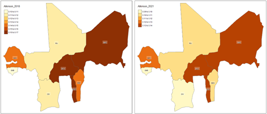
Figure 9: National level distribution of household consumption inequality within WAEMU, based on the indices of Gini

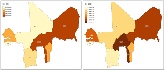
Figure 10: National level distribution of household consumption inequality growth rates between 2018 and 2021 within WAEMU, based on the indices of Atkinson (left panel) and Gini (right panel)

Regional Monitoring of Household Poverty within WAEMU

For the within-country regional analysis of household poverty, we rely on the static and dynamic graphical control charts for regional poverty monitoring shown in Figures 11–15. Starting with the indices of Watts summarized in Figure 11, from the left panel representing the data for 2018, we observe a mean Watts index value of 0.0595, indicating relatively low poverty levels across WAEMU regions on average. However, significant regional disparities are evident, with the index ranging from a minimum of 0 in Dakar, Senegal (indicating no poverty) to a maximum of 0.2561 in Savanes, Togo.

By 2021, the Watts index increased to an average of 0.0797, suggesting a general rise in poverty levels. The index ranged from 0.0003 to 0.2708, with a standard deviation of 0.0643, indicating persistent and even slightly increased variability in poverty levels across regions compared to 2018.

Similar patterns are observed with the Sen poverty index in Figure 12. The Sen index for 2018 had an average value of 0.0636. By 2021, the Sen index increased to an average of 0.0846, with persistent regional outliers experiencing extreme poverty (e.g. the “Savanes” region in Togo, the “Nord” region in Burkina Faso, and the “Maradi” region in Niger).

Additional insights from the regional monitoring of household poverty are obtained from the Foster indices (α = 0 and α = 1). The Foster index with α = 0 reflects the proportion of the population below the poverty line, representing “poverty incidence”. By 2021, the average Foster index (α = 0) rose slightly to 6.5657, suggesting a modest increase in poverty incidence across WAEMU.

The Foster index with α = 1 accounts for the depth of poverty, giving more weight to poorer individuals, representing poverty severity. By 2021, the average Foster index (α = 1) increased to 0.2409, indicating worsening poverty severity across WAEMU.

Figure 11: Regional level distribution of household poverty within WAEMU, based on the indices of Watts

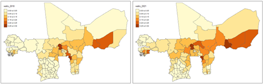
Figure 12: Regional level distribution of household poverty within WAEMU, based on the indices of Sen

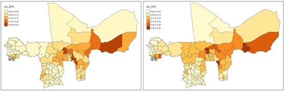
Figure 13: Regional level distribution of household poverty incidence within WAEMU, based on the indices of Foster (α = 0)

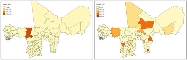
Figure 14: Regional level distribution of household poverty severity within WAEMU, based on the indices of Foster (α = 1)

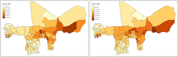
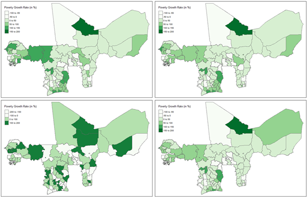
Figure 15: Regional level distribution of the household poverty growth rates between 2018 and 2021 within WAEMU, based on the indices of Watts (top-left), Sen (top-right), Foster0 (bottom-left) and Foster1 (bottom-right)

National Monitoring of Household Poverty within WAEMU

For the between-country national monitoring of household poverty in WAEMU, we rely on the static and dynamic graphical control charts shown in Figures 16–20. The comprehensive analysis using the indices of Watts, Sen, and Foster (α = 0 and α = 1), reveals critical insights into poverty incidence, severity, inequality, and depth. The 2018 state of nature highlights moderate poverty levels across the 8 WAEMU countries, with considerable variability. For instance, the average national poverty incidence, as measured by the Watts index, was 0.0712, with the lowest value in Senegal (0.0193) and the highest in Niger (0.1286).

By 2021, poverty levels rose slightly across most indices. For example, the average Watts index value increased to 0.0930, with Niger (0.1666) and Senegal (0.0366) marking the extremes.

The results from the contemporaneous cumulative state of nature ANOVA test indicate that as of 2021, the average poverty incidence significantly varies across WAEMU countries (Watts: F(7,95) = 9.711, p < 0.001; Sen: F(7,95) = 9.774, p < 0.001). Additionally, based on the Foster’s Index with α = 1, the contemporaneous ANOVA test confirmed the significant differences in poverty severity across WAEMU member states in 2021 (F(7,95) = 8.812, p < 0.001).

The second ANOVA test on the growth rates of the poverty indices revealed significant differences in average poverty incidence growth rates for the Watts Index (F(7,95) = 3.927, p < 0.001) and Sen Index (F(7,95) = 4.035, p < 0.001). Follow-up Tukey HSD post-hoc testing identified specific country pairs with significant differences in growth rates. For instance, Senegal exhibited a significantly higher poverty incidence growth rate than Burkina Faso (Watts: diff = 67.94, p = 0.011; Sen: diff = 66.48, p = 0.007).

Figure 16: National level distribution of household poverty within WAEMU, based on the indices of Watts

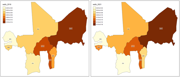
Figure 17: National level distribution of household poverty within WAEMU, based on the indices of Sen

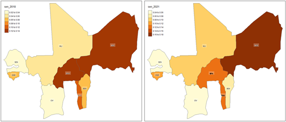
Figure 18: National level distribution of household poverty incidences within WAEMU, based on the indices of Foster (α = 0)

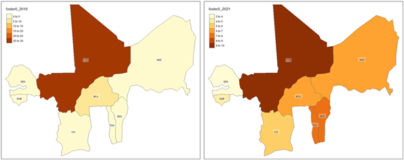
Figure 19: National level distribution of household poverty severity within WAEMU, based on the indices of Foster (α = 1)

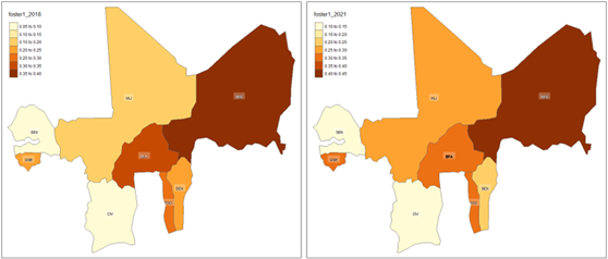
Figure 20: National level distribution of the household poverty growth rates between 2018 and 2021 within WAEMU, based on the indices of Watts (top-left), Sen (top-right), Foster0 (bottom-left) and Foster1 (bottom-right)

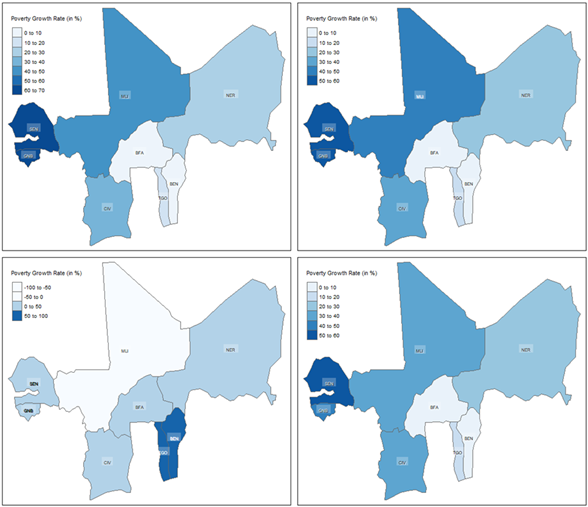
Findings from the Multivariate Conditional Monitoring Scheme (MPLPMS)

Penalized Maximum Likelihood Estimation (PMLE) was employed to estimate the parameters of the multivariate partially linear Gaussian Copula-based profile monitoring system. The algorithm evaluated the conditional consumption dynamics, identifying the impacts of key drivers across the five interdependent equations shown in the algorithmic calibration section.

Findings from the Estimated Conditional Mean Functions

Conditional Mean Food Consumption Function

The findings from the conditional mean food consumption monitoring reveal important demographic, socio-economic, as well as Spatio-temporal drivers of household average food-consumption behaviour within WAEMU. Demographic factors such as gender, revealed male-headed households with 4.89% significantly higher average food consumption spending than their female-headed counterparts within WAEMU. Additionally, the age of household head demonstrates strong non-linear effects (\text{edf} = 9.00, p < 0.001), emphasizing its significant influence on household average food consumption spending (see top-left panel in Figure 21). Moreover, regarding the influences of marital status, relative to those never married, polygamous households are found to exhibit the highest average food consumption spending (18.07%). Furthermore, compared to their counterparts with no religious beliefs, Muslim and Christian households show respective 7.29% and 3.21% higher average food consumption spending, while Animist households show 2.55% lower average food consumption spending. Larger households are also found to record 8.17% higher average food consumption, for every person increase in household size.

Regarding the impact of socio-economic factors, findings reveal that higher educational achievement by a household head positively affects a household’s average food consumption spending by 21.69%. This positive impact on household average food consumption drops to 9.88% and 7.00% respectively for secondary and primary educational achievements, compared to households with heads reporting no education. The acquisition of diploma certificates appears to amplify these average food consumption effects by 15.99% for households with heads reporting at least a university diploma.

With regard to the impact of short-term employment and economic activity, the findings show that households with heads reporting activity during the week prior to the data collection, highlight respectively 8.28% and 11.88% higher average food consumption spending than their counterparts with unemployed and inactive heads in the WAEMU labour market.

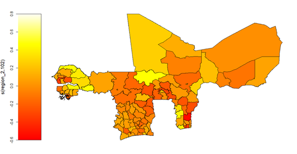
Concerning the influences of temporal and spatial factors on household average food wellness within WAEMU, the findings revealed a 16.54% annual increase in average food consumption spending between 2020 and 2021. Spatially, urban households exhibited 18.06% higher average food consumption spending compared to their rural counterparts. As shown in Figure 22, significant non-linear and spatially heterogenous average food consumption spending was also recorded across the 103 administrative regions (\text{edf} = 102, p < 0.001) within WAEMU.

Figure 21: Smooth function plots of the age (left panel), random country of origin (central panel), and random country of residence (right panel) effects on household mean food consumption spending (top panels), and mean non-food consumption spending (lower panels) within WAEMU

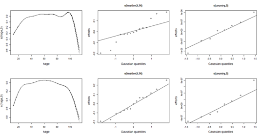
Figure 22: Conditional Heterogeneity in household Mean Food consumption spending (Food Wellness mean heterogeneity across regions) within WAEMU

Conditional Mean Non-Food Consumption Function

Similar to the mean food consumption spending described above, demographic factors such as gender revealed that male-headed households show positive and significantly higher (5.90%) average non-food consumption spending than their female-headed counterparts within WAEMU. Additionally, household head’s age shows an inverted-U effect (\text{edf} = 8.99, p < 0.001), emphasizing its significant non-linear influence on household average non-food consumption spending (see bottom-left panel in Figure 21).

Regarding the impact of socio-economic factors, findings revealed that higher educational achievement by a household head positively affects a household’s average non-food consumption by 37.68%. This positive impact on household average non-food consumption spending drops to 20.03% and 15.76% respectively for secondary and primary educational achievements, compared to households with heads reporting no education. The acquisition of diploma certificates appears to also amplify these average non-food consumption effects by 50.92% for households with heads reporting at least a university diploma.

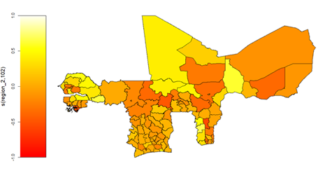
Concerning the influences of temporal and spatial factors, the findings revealed 11.41% yearly increases in average non-food consumption between 2018 and 2021 within WAEMU. Spatially, compared to their rural counterparts, urban households exhibited 29.58% higher average non-food consumption spending. As shown in Figure 23, significant non-linear (\text{edf} = 102, p < 0.001) and spatially heterogenous average non-food consumption spending was also recorded across the 103 administrative regions within WAEMU.

Figure 23: Conditional Heterogeneity in household Mean non-Food consumption spending (non-Food Wellness mean heterogeneity across regions) within WAEMU

Findings from the Estimated Conditional Variance-Covariance Functions

The monitoring scheme also integrates findings from the conditional variance and covariance functions to provide further understanding of household food and non-food consumption dynamics within WAEMU.

Conditional Variance of Food Consumption

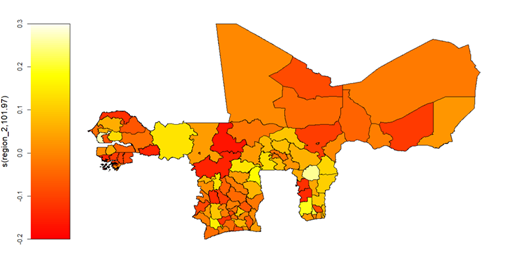
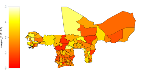
The monitoring results from the conditional variance of household food consumption reveal significant spatial and temporal factors with non-linear influences on household food-consumption spending variations within WAEMU. In the temporal domain, the findings highlight a 7.22% reduced variation in household annual food-consumption spending between 2018 and 2021. Additionally, significant food consumption seasonality is recorded within WAEMU, with wave 2 interviewed households showing 6.57% lower variations in food-consumption spending than their wave 1 counterparts.

Figure 24: Conditional Heterogeneity in household Variance of Food consumption spending within WAEMU

Figure 24: Conditional heterogeneity in household variance of food consumption spending (Food Wellness variance heterogeneity across regions) within WAEMU.

Conditional Variance of Non-Food Consumption

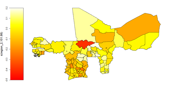
The monitoring results from the conditional variance of household non-food consumption also reveal key spatial and temporal factors driving household non-food consumption behaviour variations within WAEMU. Temporally, a 2.76% reduced variation emerges in household annual non-food consumption spending between 2018 and 2021. Also, a significant non-food consumption seasonality seems to prevail within WAEMU, with wave 2 interviewed households showing 5.38% lower variations in non-food consumption spending than their wave 1 counterparts.

Figure 25: Conditional Heterogeneity in household Variance of non-Food consumption spending within WAEMU

Figure 25: Conditional heterogeneity in household variance of non-food consumption spending (non-Food Wellness variance heterogeneity across regions) within WAEMU.

Conditional Covariance between Food and Non-Food Consumption

The monitoring results from the conditional co-variance between household food and non-food consumption also highlight important spatial and temporal factors driving the inter-dependence of household behaviour towards food and non-food consumption within WAEMU. In the temporal dimension, we note a 3.13% higher co-variation between household annual food and non-food consumption spending in 2021, compared to 2018. Additionally, seasonal effects also exist, with second wave interviewed households showing 1.25% higher co-variations between food and non-food consumption spending, than their first wave counterparts.

Figure 26: Conditional Heterogeneity in household Co-Variance between Food and Non-food consumption spending within WAEMU

Figure 26: Conditional heterogeneity in household co-variance between food and non-food consumption spending (Food and non-food Wellness co-variance heterogeneity across regions) within WAEMU.

Predicted Findings from the Fitted Multivariate Conditional Monitoring Scheme

The observed heterogeneities in the means and variance-covariance parameters depicted from Figures 22 to 26, follow penalized maximum likelihood estimation of the multivariate partially linear Gaussian Copula profile monitoring system. These heterogeneities suggest that after controlling for factors driving households’ annual food and non-food expenditures dynamics within WAEMU, important differences still remain in the spatial variations and covariations of household food and non-food wellness, between and within WAEMU states.

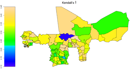
The algebraic results of the point and interval estimations of these remaining unexplained variations, reveal an overall WAEMU level average, post-estimation conditional variance of household food consumption spending of 0.511 (or 51.1%) with a 95% C.I. of (0.510, 0.512), which are further regionally depicted in Figure 27. Similarly, the overall WAEMU level conditional variance of household non-food consumption spending is 0.55 (or 55%) with 95% C.I. (0.548, 0.551) and is also regionally depicted in Figure 28. Moreover, the post-estimation conditional covariance parameter is predicted as \hat{\rho} = 0.518 (95% C.I.: 0.516, 0.521), along with the Kendall’s \tau parameter = 0.348 (0.346, 0.350), which captures the dependence between the two Gaussian Copula margins of households’ food and non-food consumption spending, as regionally depicted in Figure 29.

Figure 27: Predicted administrative regional level variations in household Food consumption spending within WAEMU

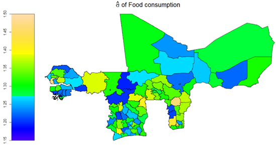
Figure 28: Predicted administrative regional level variations in household consumption spending on non-food items within WAEMU

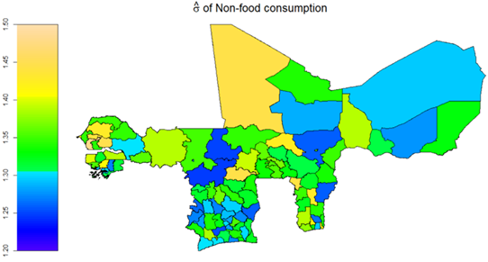
Figure 29: Predicted administrative regional level degree of dependence between household consumption spending on food and non-food items within WAEMU

Discussions and Implications

Results Discussions

The results of this study provide a novel perspective on the application of process monitoring methodologies to household consumption processes within regional economic blocs, with a particular focus on the West African Economic and Monetary Union (WAEMU). By leveraging the EHCVM data, this study developed and implemented for the first time in the literature, a multivariate partially linear profile monitoring system (MPLPMS) that tracks household food and non-food consumption patterns over time. The findings underscore the utility of employing statistical process monitoring (SPM) frameworks (Ghasemi et al., 2023; Haq & Ali, 2024), particularly the combination of univariate and multivariate schemes (Sabahno et al., 2020; Sabahno & Amiri, 2023), to identify deviations in household consumption patterns that are indicative of broader socio-economic disparities.

Unconditional Monitoring Scheme Results

The unconditional monitoring of inequality and poverty dynamics reveals baseline critical insights into household food and non-food consumption patterns within WAEMU. The findings from the adopted graphical control charts emphasized spatial and temporal dimensions of consumption disparities, persistent vulnerabilities, and a growing urgency for comprehensive, targeted, and regionally coordinated policy interventions for achieving equitable economic outcomes.

For instance, the unconditional monitoring scheme reveals stark inequality dynamics both within administrative regions and across countries. Certain administrative regions, such as those in Niger and Guinea-Bissau, exhibit higher levels of inequality as measured by the Gini and Atkinson indices. Temporal trends indicate that inequality has generally increased between 2018 and 2021, albeit with variability across regions.

The findings also shed light on significant poverty disparities within administrative regions and across countries. Regions in Niger and Guinea-Bissau exhibit high poverty incidence and severity, as evidenced by the Watts, Sen, and Foster indices. Nationally, cross-country disparities in poverty levels are striking. Niger recorded the highest poverty incidence and severity in 2021, while Senegal consistently displayed the lowest levels. The statistical significance of these disparities, confirmed through ANOVA testing, underscores the urgency for differentiated national strategies and regional cooperation.

Consequently, the interplay between inequality and poverty within administrative regions highlights the need for integrated policy approaches. Moreover, the unconditional monitoring scheme underscores the importance of coordinated WAEMU-wide policies. This latter suggestion is also consistent with reports from the EU context, where funding decreased social exclusion, especially in Eastern European countries (Ferraro et al., 2021).

Multivariate Conditional Monitoring Scheme Results Discussions

Meanwhile, the multivariate partially linear conditional monitoring scheme enriched the analysis by incorporating the interdependencies and conditional dynamics between food and non-food consumption, using semi-parametric copula regression methods. Results from the conditional mean functions revealed intricate demographic, socio-economic, spatial, and temporal drivers influencing household average consumption expenditures.

Indeed, consistent with the importance of considering gender dynamics in food expenditure analyses reported in Jagannarayan & Prasuna (2024), gender differences were evident in this study, with male-headed households exhibiting higher average food and non-food consumption spending compared to female-headed households. Additionally, corroborating recent reports from E. Lee et al. (2024) and Madudova & Corejova (2023), household size demonstrated a positive relationship with average consumption, emphasizing economies of scale in larger households. Aligned also with the rural-urban welfare gaps reported in Ghana (Tawiah et al., 2024), our findings revealed urban households to consistently record higher average spending on both food and non-food items compared to their rural counterparts.

Temporal trends revealed annual increases in household average consumption spending, underscoring potential economic recovery or growth dynamics during the 2021 fiscal year, compared to the post-pandemic period of 2018. This finding is consistent with Baker et al. (2020), which found over 40% increased spending among US households, during the first half of March 2020, followed by a 25% to 30% decreased in overall spending as the pandemic spread. It also corroborates Yannelis & Amato (2023), which reported the pandemic to have induced an initial decline in consumption, subsequently followed by a rapid rebound.

Moreover, consistent with the results based on OLS with Random Forest regressions (E. Lee et al., 2024), education and employment emerged in this study as critical socio-economic determinants, with higher educational attainment and active labor market participation positively driving household average consumption. Furthermore, spatial heterogeneity in household average consumption spending, highlighted by significant regional disparities, underscores the necessity for localized policy interventions. These are consistent with Lichner et al. (2022), which relying on \sigma-convergence and \beta-convergence frameworks, reported the joint evaluation of income and consumption to be crucial for understanding regional economic imbalances.

Finally, the estimated conditional variance and covariance functions highlighted critical spatial and temporal dynamics. The observed dependencies between food and non-food consumption spending underscore the interconnected nature of household decision-making, which is influenced by systemic and idiosyncratic factors.

Research Implications

Theoretical Implications

The study contributes significantly to the theoretical landscape by integrating unconditional and multivariate conditional approaches, thereby expanding the scope of process monitoring research to encompass economic processes, particularly household consumption within regional economic blocs. This approach represents a paradigm shift from the traditional focus on industrial and manufacturing processes to the broader socio-economic context. By conceptualizing household consumption as a regional process profile, the study bridges a critical gap in the literature, integrating insights from quality control and statistical monitoring into the realm of economic analysis.

The study also advances the theoretical framework by highlighting the interconnectedness of food and non-food consumption, as captured by the Gaussian Copula-based profile monitoring system. This interdependence challenges traditional separations of household budget allocations and necessitates a holistic perspective on household consumption behavior research.

Methodological Implications

Methodologically, the study pioneers the application of a multivariate partially linear profile monitoring system (MPLPMS) to regional household consumption processes. The integration of univariate and multivariate schemes within a single framework represents a significant advancement in process monitoring methodologies. The use of semi-parametric multivariate copula regression enhances the flexibility and robustness of the monitoring system, allowing for the simultaneous tracking of mean and variance-covariance parameters.

Overall, the use of Penalized Maximum Likelihood Estimation (PMLE) within the multivariate partially linear Gaussian Copula profile monitoring system demonstrates the effectiveness of advanced statistical process control methods in capturing complex consumption dynamics. In addition to its value as a continuous consumption monitoring system for the West African Economic and Monetary Union, the developed methodological framework can serve as a benchmark template for similar analyses in other regions or contexts.

General Policy Implications

This research has profound implications for general policy design and implementation. In fact, the study’s focus on household consumption as a critical component of economic activity underscores the importance of integrating consumption monitoring into broader development strategies. Its univariate and multivariate schemes combine to not only provide a robust framework for household consumption patterns monitoring, but also offer actionable insights into key drivers of poverty and inequality, thereby enabling targeted policy interventions.

Overall, several policy priorities transpire for the WAEMU bloc, based on the applied findings from the framework in this study. These including: (i) addressing gender disparities, with policies that focus on empowering female-headed households through targeted financial support, education, and employment opportunities to bridge the consumption gap; (ii) enhancing educational access through investments in education, particularly at higher levels, would significantly increase household consumption, thereby improving overall welfare; (iii) strengthening labour market participation, with policies promoting employment opportunities and labour market integration, especially for rural and inactive populations, would also enhance household consumption capacity; (iv) reducing spatial inequalities, through regional development programs that address structural disparities and enhance resource allocation in less developed regions; and (v) instilling seasonal support mechanisms, through targeted interventions during periods of high consumption vulnerability to mitigate seasonal effects and stabilize household welfare.

Implications for the United Nations Sustainable Development Goals (SDGs)

The research findings align closely with the United Nations Sustainable Development Goals (SDGs), particularly SDG 1 (No Poverty), SDG 2 (Zero Hunger), SDG 5 (Gender Equality), SDG 8 (Decent Work and Economic Growth), SDG 10 (Reduced Inequalities), and SDG 12 (Responsible Consumption and Production). By providing a comprehensive framework for monitoring household consumption patterns, the study directly contributes to efforts aimed at eradicating poverty and hunger, reducing inequalities, and promoting sustainable consumption practices.

Indeed, the univariate and multivariate monitoring schemes offer actionable insights for tracking progress toward these goals. For example, the identification of regions with high levels of food consumption inequality could inform initiatives to enhance food security and nutrition (Goals 2 and 10). Similarly, the monitoring of non-food consumption patterns could support efforts to improve access to education, healthcare, and other essential services, fostering inclusive and sustainable development within WAEMU states (Goals 8 and 12). Overall, the study and its findings provide a scalable and replicable framework for advancing the UN global agenda for sustainable development.

Conclusion and Future Research Suggestions

Summary of Research Contributions

This study pioneers a novel integration of statistical process monitoring and regional household consumption analysis, offering a framework to monitor and analyze regional economic level (WAEMU) food and non-food consumption dynamics. By applying profile monitoring techniques, such as the multivariate partially linear profile monitoring system (MPLPMS) and copula-based regression, this research bridges the gap between traditional process monitoring in manufacturing and service sectors and broader socio-economic contexts. Specifically, the study:

Introduces the concept of regional consumption process monitoring to capture complex economic behaviors in a regional economic bloc setting.
Develops simultaneous monitoring schemes for tracking consumption parameters, addressing both unconditional (poverty and inequality indices) and conditional (spatial and temporal influences) profiles.
Provides actionable insights into the drivers of household consumption behavior, offering a comprehensive understanding of how poverty and inequality evolve across WAEMU.
Contributes to policymaking by presenting practical, data-driven solutions aligned with the UN Sustainable Development Goals (SDGs).

By expanding the scope of profile monitoring to regional economic processes, this study contributes methodologically to the literature and practically to the policy discourse in developing regions. While it presents significant advancements, this research is not without limitations. For instance, the analysis relies on the EHCVM survey, which, while comprehensive, provides data at only two-year intervals and may not fully capture real-time consumption changes or nuanced socio-economic dynamics. Additionally, while the WAEMU region is an exemplary case, the findings may not be directly generalizable to other regional blocs with differing socio-economic structures and governance frameworks. Moreover, the use of semi-parametric multivariate copula regression, while robust, requires extensive computational resources and expertise, potentially limiting its replicability in regions with less access to advanced tools, and computational power. Finally, in its current development, the study primarily focuses on economic indicators of consumption, omitting potentially significant behavioral, cultural, and psychological drivers of household consumption.

Future Research Suggestions

Building on the study’s contributions and addressing its identified limitations, several avenues of fruitful future research directions emerge. For instance, to expend temporal resolution, future studies could incorporate higher-frequency or real-time data collection mechanisms, such as mobile-based surveys or digital transaction records that better capture short-term consumption dynamics. Additionally, the adopted methodologies could be applied to other regional economic blocs, such as the Southern African Development Community (SADC) or the Association of Southeast Asian Nations (ASEAN), to assess the universality and adaptability of the framework. Moreover, future research could

References

Acar, P., & Sundararaghavan, V. (2016). A Markov random field approach for modeling spatio-temporal evolution of microstructures. Modelling and Simulation in Materials Science and Engineering, 24(7), 075005. https://doi.org/10.1088/0965-0393/24/7/075005

Aguilera, A. M., & Aguilera-Morillo, M. C. (2013). Comparative study of different B-spline approaches for functional data. Mathematical and Computer Modelling, 58(7–8), 1568–1579. https://doi.org/10.1016/j.mcm.2013.04.007

Ahmadi Yazdi, A., Shafiee Kamalabad, M., Oberski, D. L., & Grzegorczyk, M. (2024). Bayesian multivariate control charts for multivariate profiles monitoring. Quality Technology & Quantitative Management, 21(3), 386–421. https://doi.org/10.1080/16843703.2023.2201537

Amir, W. A. F. W., Misro, M. Y., & Mohd, M. H. (2024). Flexible functional data smoothing and optimization using beta spline. AIMS Mathematics, 9(9), 23158–23181. https://doi.org/10.3934/math.20241126

Atkinson, A. B. (1996). The distribution of income: Evidence, theories and policy. De Economist, 144(1), 1–21. https://doi.org/10.1007/BF01680329

Baker, S. R., Farrokhnia, R. A., Meyer, S., Pagel, M., & Yannelis, C. (2020). How does household spending respond to an epidemic? Consumption during the 2020 COVID-19 pandemic. The Review of Asset Pricing Studies, 10(4), 834–862. https://doi.org/10.1093/rapstu/raaa009

Bigsten, A. (2024). Atkinson on inequality. In Inequality: Economic and social issues (pp. 95–111). Springer.

Busababodhin, P., & Amphanthong, P. (2016). Copula modelling for multivariate statistical process control: A review. Communications for Statistical Applications and Methods, 23(6), 497–515. https://doi.org/10.5351/CSAM.2016.23.6.497

Cowell, F. A. (2000). Measurement of inequality. Handbook of Income Distribution, 1, 87–166. https://doi.org/10.1016/S1574-0056(00)80005-6

Cowell, F. A. (2015). Income distribution and inequality. In The elgar companion to social economics, second edition (pp. 235–252). Edward Elgar Publishing.

Easton, A., Dalen, O. van, Goeb, R., & Di Bucchianico, A. (2022). Bivariate copula monitoring. Quality and Reliability Engineering International, 38(3), 1272–1288. https://doi.org/10.1002/qre.3025

Eilers, P. H. C., & Marx, B. D. (1996). Flexible smoothing with B-splines and penalties. Statistical Science, 11(2), 89–121. https://doi.org/10.1214/ss/1038425655

Faton, A. K., & Chabossou, A. (2024). Digital financial inclusion and household consumption expenditure in ECOWAS. Journal of African Development, 26(1), 1–20.

Fellman, J. (2012). Estimation of Gini coefficients using Lorenz curves. Journal of Statistical and Econometric Methods, 1(2), 31–38.

Ferraro, A., Cerciello, M., Agovino, M., & Garofalo, A. (2021). Do public policies reduce social exclusion? The role of national and supranational economic tools. Structural Change and Economic Dynamics, 57, 165–181. https://doi.org/10.1016/j.strueco.2021.04.005

Foster, J. E. (1984). On economic poverty: A survey of aggregate measures. Advances in Econometrics, 3, 215–251.

Foster, J., Greer, J., & Thorbecke, E. (2010). The Foster–Greer–Thorbecke (FGT) poverty measures: 25 years later. The Journal of Economic Inequality, 8, 491–524. https://doi.org/10.1007/s10888-010-9136-1

García-Gómez, C., Pérez, A., & Prieto-Alaiz, M. (2021). Copula-based analysis of multivariate dependence patterns between dimensions of poverty in Europe. Review of Income and Wealth, 67(1), 165–195. https://doi.org/10.1111/roiw.12436

Gastwirth, J. L. (1972). The estimation of the Lorenz curve and Gini index. The Review of Economics and Statistics, 306–316. https://doi.org/10.2307/1937992

Ghasemi, Z., Zeinal Hamadani, A., & Ahmadi Yazdi, A. (2023). New methods for phase II monitoring of multivariate simple linear profiles. Communications in Statistics – Simulation and Computation, 1–25. https://doi.org/10.1080/03610918.2022.2162797

Haq, A., & Ali, Q. (2024). A maximum dual CUSUM chart for joint monitoring of process mean and variance. Quality Technology & Quantitative Management, 21(3), 287–308. https://doi.org/10.1080/16843703.2023.2188912

Jagannarayan, M. N., & Prasuna, A. (2024). Gender (Women-Led households) as a determinant of consumption expenditure on food during March 2020 – A case study of Maharashtra. South Eastern European Journal of Public Health, 269–276.

Jalilibal, Z., Amiri, A., & Khoo, M. B. C. (2022). A literature review on joint control schemes in statistical process monitoring. Quality and Reliability Engineering International, 38(6), 3270–3289. https://doi.org/10.1002/qre.3128

Jenkins, S. P. (2017). The measurement of income inequality. In Economic inequality and poverty (pp. 3–38). Routledge.

Kamble, P., Mehta, A., & Rani, N. (2024). Financial inclusion and digital financial literacy: Do they matter for financial well-being? Social Indicators Research, 171(3), 777–807. https://doi.org/10.1007/s11205-023-03271-5

Krupskii, P., Harrou, F., Hering, A. S., & Sun, Y. (2020). Copula-based monitoring schemes for non-Gaussian multivariate processes. Journal of Quality Technology, 52(3), 219–234. https://doi.org/10.1080/00224065.2019.1571342

Kuznets, S. (2019). Economic growth and income inequality. In The gap between rich and poor (pp. 25–37). Routledge.

Lee, E., Ong, T. S., & Lee, Y. (2024). Evaluating household consumption patterns: Comparative analysis using Ordinary Least Squares and Random Forest regression models. HighTech and Innovation Journal, 5(2), 489–507. https://doi.org/10.28991/HIJ-2024-05-02-018

Lee, K.-K. (2014). Globalization, income inequality and poverty: Theory and empirics. Social System Studies, 28, 109–134.

Lichner, I., Lyócsa, Š., & Výrostová, E. (2022). Nominal and discretionary household income convergence: The effect of a crisis in a small open economy. Structural Change and Economic Dynamics, 61, 18–31. https://doi.org/10.1016/j.strueco.2021.11.006

Lindgren, F., Rue, H., & Lindström, J. (2011). An explicit link between Gaussian fields and Gaussian Markov random fields: The stochastic partial differential equation approach. Journal of the Royal Statistical Society Series B: Statistical Methodology, 73(4), 423–498. https://doi.org/10.1111/j.1467-9868.2011.00777.x

Liu, Q., Yu, M., & Wang, X. (2015). Poverty reduction within the framework of SDGs and Post-2015 development agenda. Advances in Climate Change Research, 6(1), 67–73. https://doi.org/10.1016/j.accre.2015.09.004

Madudova, E., & Corejova, T. (2023). The issue of measuring household consumption expenditure. Economies, 12(1), 9. https://doi.org/10.3390/economies12010009

Mahendra, I. G. B. (2024). Addressing the inequality in the Sustainable Development Goals (SDGs) globally. Journal of Public Health, fdae199. https://doi.org/10.1093/pubmed/fdae199

Marra, G., & Radice, R. (2017). Bivariate copula additive models for location, scale and shape. Computational Statistics & Data Analysis, 112, 99–113. https://doi.org/10.1016/j.csda.2017.03.004

Marra, G., & Radice, R. (2024). Generalized joint regression modelling – GJRM. CRAN packages version 0.2-6.7. https://doi.org/10.32614/CRAN.package.GJRM

Mayr, A., Fenske, N., Hofner, B., Kneib, T., & Schmid, M. (2012). Generalized additive models for location, scale and shape for high dimensional data – a flexible approach based on boosting. Journal of the Royal Statistical Society Series C: Applied Statistics, 61(3), 403–427. https://doi.org/10.1111/j.1467-9876.2011.01033.x

Nai Ruscone, M. (2024). Copula-based measures of association. In Encyclopedia of quality of life and well-being research (pp. 1420–1425). Springer International Publishing.

Naveenan, R. V., Liew, C. Y., & Kijkasiwat, P. (2024). Nexus between financial inclusion, digital inclusion and health outcomes: Evidence from developing economies. Social Indicators Research, 174(1), 367–408. https://doi.org/10.1007/s11205-024-03327-y

Nghiem, N., Teng, A., Cleghorn, C., McKerchar, C., & Wilson, N. (2022). Using household economic survey data to assess food expenditure patterns and trends in a high-income country with notable health inequities. Scientific Reports, 12(1), 1–9. https://doi.org/10.1038/s41598-022-07222-3

Niankara, I. (2022). Sustainability through open data sharing and reuse in the digital economy. 2022 International Arab Conference on Information Technology (ACIT), 1–11. https://doi.org/10.1109/ACIT57182.2022.9994191

Niankara, I. (2023). Socioeconomic and geospatial determinants of households’ food and non-food consumption dynamics within the West African Economic and Monetary Union. Scientific African, 20, e01724. https://doi.org/10.1016/j.sciaf.2023.e01724

Niankara, I., Refae, G. A. E., & Qasim, A. (2023). A spatial bivariate copula regression analysis of youths’ access to ICT resources and subjective well-being in the Middle East. International Journal of Economics and Business Research, 26(1), 43–83. https://doi.org/10.1504/IJEBR.2023.132154

Ogwang, T. (2022). The Foster–Greer–Thorbecke poverty measures reveal more. Social Indicators Research, 164(3), 1481–1503. https://doi.org/10.1007/s11205-022-02989-y

Perperoglou, A., Sauerbrei, W., Abrahamowicz, M., & Schmid, M. (2019). A review of spline function procedures in R. BMC Medical Research Methodology, 19, 1–16. https://doi.org/10.1186/s12874-019-0666-3

Programme d’Harmonisation et de Modernisation des Enquêtes sur les Conditions de Vie des ménages (PHMECV). (2023). Enquête harmonisée sur le conditions de vie des ménages (EHCVM), all 8 WAEMU country members 2018/2019 (1st Ed.) And 2021/2022 (2nd Ed.) – panel surveys.

R Core Team. (2024). R: A language and environment for statistical computing. R Foundation for Statistical Computing. https://www.R-project.org/

Rahimi, S. B., Amiri, A., Khoo, M. B. C., & Shadman, A. (2022). Simultaneous monitoring of mean vector and covariance matrix of auto-correlated multivariate multiple linear profiles. Quality and Reliability Engineering International, 38(7), 3513–3542. https://doi.org/10.1002/qre.3149

Robeyns, I. (2005). The capability approach: A theoretical survey. Journal of Human Development, 6(1), 93–117. https://doi.org/10.1080/146498805200034266

Russell, J., Lechner, A., Hanich, Q., Delisle, A., Campbell, B., & Charlton, K. (2018). Assessing food security using household consumption expenditure surveys (HCES): A scoping literature review. Public Health Nutrition, 21(12), 2200–2210. https://doi.org/10.1017/S136898001800068X

Sabahno, H., & Amiri, A. (2023). Simultaneous monitoring of the mean vector and covariance matrix of multivariate multiple linear profiles with a new adaptive Shewhart-type control chart. Quality Engineering, 35(4), 600–618. https://doi.org/10.1080/08982112.2023.2195200

Sabahno, H., Castagliola, P., & Amiri, A. (2020). An adaptive variable-parameters scheme for the simultaneous monitoring of the mean and variability of an autocorrelated multivariate normal process. Journal of Statistical Computation and Simulation, 90(8), 1430–1465. https://doi.org/10.1080/00949655.2020.1726686

Sancetta, A., & Satchell, S. (2004). The Bernstein copula and its applications to modeling and approximations of multivariate distributions. Econometric Theory, 20(3), 535–562. https://doi.org/10.1017/S026646660420306X

Schmelzer, B. (2015). Joint distributions of random sets and their relation to copulas. International Journal of Approximate Reasoning, 65, 59–69. https://doi.org/10.1016/j.ijar.2015.04.009

Sen, A. (1993). Capability and well-being. In The quality of life (Vol. 30, pp. 270–293). Clarendon Press.

Shorrocks, A. F. (1995). Revisiting the Sen poverty index. Econometrica: Journal of the Econometric Society, 1225–1230. https://doi.org/10.2307/2171728

Sklar, A. (1973). Random variables, joint distribution functions, and copulas. Kybernetika, 9(6), 449–460.

Smith, M. S. (2023). Implicit copulas: An overview. Econometrics and Statistics, 28, 81–104. https://doi.org/10.1016/j.ecosta.2021.08.004

Song, Z., Mukherjee, A., & Zhang, J. (2021). Some robust approaches based on copula for monitoring bivariate processes and component-wise assessment. European Journal of Operational Research, 289(1), 177–196. https://doi.org/10.1016/j.ejor.2020.06.047

Stasinopoulos, D. M., & Rigby, R. A. (2008). Generalized additive models for location scale and shape (GAMLSS) in R. Journal of Statistical Software, 23, 1–46. https://doi.org/10.18637/jss.v023.i07

Tasias, K. A., & Nenes, G. (2012). A variable parameter Shewhart control scheme for joint monitoring of process mean and variance. Computers & Industrial Engineering, 63(4), 1154–1170. https://doi.org/10.1016/j.cie.2012.06.021

Tawiah, T. O., Sakyi, D., Ayibor, R. E., & Amanor, K. (2024). The impact of financial inclusion on rural–urban households welfare inequality in Ghana: A decomposition analysis. Review of Development Economics. https://doi.org/10.1111/rode.13133

Thiombiano, N., Ouedraogo, S., & Moussa, A. (2022). Fiscal policy rules and economic fluctuations in the countries of the West African Economic and Monetary Union (WAEMU). Research in Economics, 76(3), 252–263. https://doi.org/10.1016/j.rie.2022.07.003

Trivedi, P. K., & Zimmer, D. M. (2007). Copula modeling: An introduction for practitioners. In Foundations and Trends in Econometrics (Vol. 1, pp. 1–111). Now Publishers. https://doi.org/10.1561/0800000005

Vatter, T., & Chavez-Demoulin, V. (2015). Generalized additive models for conditional dependence structures. Journal of Multivariate Analysis, 141, 147–167. https://doi.org/10.1016/j.jmva.2015.07.003

Vatter, T., & Nagler, T. (2018). Generalized additive models for pair-copula constructions. Journal of Computational and Graphical Statistics, 27(4), 715–727. https://doi.org/10.1080/10618600.2018.1451338

Verdier, G. (2013). Application of copulas to multivariate control charts. Journal of Statistical Planning and Inference, 143(12), 2151–2159. https://doi.org/10.1016/j.jspi.2013.08.003

Wang, F., Zhang, X., Ye, C., & Cai, Q. (2024). The household multidimensional poverty reduction effects of digital financial inclusion: A financial environment perspective. Social Indicators Research, 172(1), 313–345. https://doi.org/10.1007/s11205-023-03205-1

Wood, S. N. (2003). Thin plate regression splines. Journal of the Royal Statistical Society Series B: Statistical Methodology, 65(1), 95–114. https://doi.org/10.1111/1467-9868.00374

Wood, S. N. (2017). Generalized additive models: An introduction with R. Chapman; Hall/CRC. https://doi.org/10.1201/9781315370279

Wood, S. N., Pya, N., & Säfken, B. (2016). Smoothing parameter and model selection for general smooth models. Journal of the American Statistical Association, 111(516), 1548–1563. https://doi.org/10.1080/01621459.2016.1180986

Xu, H., Qin, W., Sun, Y., Lv, Y., & Zhang, J. (2024). An adaptive Copula function-based framework for fault detection in semiconductor wafer fabrication. Computers & Industrial Engineering, 188, 109905. https://doi.org/10.1016/j.cie.2024.109905

Yameogo, C. E., & Omojolaibi, J. A. (2022). Regional economic integration and its impact on income distribution and the poverty level: The case of the WAEMU zone. Quaestiones Geographicae, 41(2), 21–35. https://doi.org/10.2478/quageo-2022-0011

Yan, J. (2023). Multivariate modeling with copulas and engineering applications. Springer Handbook of Engineering Statistics, 931–945.

Yannelis, C., & Amato, L. (2023). Household behavior (consumption, credit, and investments) during the COVID-19 pandemic. Annual Review of Financial Economics, 15(1), 91–113. https://doi.org/10.1146/annurev-financial-110921-025428

Yao, J., Xian, X., & Wang, C. (2023). Adaptive sampling for monitoring multi-profile data with within-and-between profile correlation. Technometrics, 65(3), 375–387. https://doi.org/10.1080/00401706.2022.2134173

Yu, J., Shi, X., & Cheong, T. S. (2021). Distribution dynamics of China’s household consumption upgrading. Structural Change and Economic Dynamics, 58, 193–203. https://doi.org/10.1016/j.strueco.2021.05.009

Zaidi, F. S., Dai, H., Imran, M., & Tran, K. P. (2023). Monitoring autocorrelated compositional data vectors using an enhanced residuals Hotelling T^2 control chart. Computers & Industrial Engineering, 181, 109280. https://doi.org/10.1016/j.cie.2023.109280

Zeileis, A. (2014). ineq: Measuring inequality, concentration, and poverty.