A Complete Formal Endogenous Growth Model with Autonomous AI Innovation Agents: Theory, Equilibrium, and Simulation
We develop a complete formal endogenous growth model in which autonomous artificial intelligence (AI) agents function as independent innovators alongside human researchers, introducing computational capital as a distinct factor of production in the knowledge sector. Building on Romer (1990) and Jones (1995), our model extends the canonical knowledge-accumulation equation to incorporate superlinear agentic scaling. We fully characterise the balanced growth path, derive closed-form optimal allocations, and establish three formal propositions on AI growth acceleration, compute as a strategic asset, and innovation inequality under concentrated compute ownership.
Abstract
We develop a complete formal endogenous growth model in which autonomous artificial intelligence (AI) agents function as independent innovators alongside human researchers, introducing computational capital as a distinct factor of production in the knowledge sector. Building on Romer (1990) and Jones (1995), our model extends the canonical knowledge-accumulation equation to \dot{K}(t) = \phi_H H(t) + \phi_A [\kappa C(t)]^{\gamma}, where C(t) is computational capital, \kappa is compute-to-agent efficiency, and \gamma > 1 captures the superlinear scaling of agentic exploration. We fully characterise the model’s balanced growth path (BGP), deriving closed-form optimal allocations of human researchers and compute capital at the firm level, and establishing three formal propositions on AI growth acceleration, compute as a strategic asset, and innovation inequality under concentrated compute ownership. A Monte Carlo simulation (T = 200 periods, N = 500 firms, n = 1{,}000 draws) calibrated to OECD R&D indicators and the empirical compute-scaling literature (Babina et al., 2024; Besiroglu et al., 2024) corroborates the theoretical predictions: GDP growth accelerates by a factor of 2.1–3.8 as AI innovation dominates, while innovation Gini rises from 0.32 to 0.61 as compute concentration increases. We identify testable hypotheses linking compute investment to patent output, R&D productivity, and frontier-sector dominance, and discuss policy implications for compute governance, knowledge ownership, and AI research infrastructure.
Keywords: Endogenous growth; AI agents; computational capital; knowledge production function; Schumpeterian dynamics; Monte Carlo simulation; innovation inequality; compute governance; responsible AI; human–agent coexistence; breakthrough innovation; DAO governance.
JEL Codes: O31, O33, O41, E25, L11, D83, C63, J24.
1. Introduction
The theory of endogenous growth has, since the foundational contributions of Romer (1990) and Aghion & Howitt (1992), treated technological change as the purposeful outcome of human researchers investing in R&D under the incentive of temporary monopoly rents. In these frameworks, the fundamental constraint on long-run growth is the productivity of the human knowledge sector: ideas are produced by people, and more researchers produce more ideas, subject to the diminishing returns and “stepping on toes” effects formalised by Jones (1995) and the empirically documented difficulty of finding new ideas documented by N. Bloom et al. (2020).
That foundational assumption is now under challenge. Autonomous AI systems—capable of formulating hypotheses, designing experiments, iterating over solution spaces, and coordinating with other agents without continuous human supervision—are being deployed at scale in pharmaceutical discovery, materials science, software engineering, and mathematical research (Al-Hamad et al., 2025; Prokopowicz et al., 2025). These systems do not merely assist human researchers: they execute innovation processes that, in principle, can run continuously, in parallel, at a speed and scale bounded not by human cognitive limits but by the availability of computational infrastructure.
This paper develops a complete formal model of an economy in which AI agents function as independent innovators alongside human researchers. The model is grounded in the Romer–Jones tradition but introduces two modifications of first-order importance. First, computational capital C(t)—the stock of AI-capable hardware, trained models, and data infrastructure—enters the knowledge-production function directly, producing AI agents A(t) = \kappa C(t) that generate innovations superlinearly with their scale. Second, the firm-level R&D optimisation problem now involves choosing between two distinct innovation inputs—human researchers (priced at wage w) and compute capital (priced at rental rate r)—with differential productivity elasticities \beta and \eta respectively, where \eta > \beta encodes the AI productivity advantage at scale.
Our paper makes four contributions. First, we provide a fully-specified formal model, derive all equilibrium conditions in closed form, and prove three propositions on growth dynamics, compute substitution, and innovation concentration. Second, we develop a full Monte Carlo simulation in R that endogenises firm-level innovation decisions, calibrates parameters to empirical benchmarks, and generates growth trajectories, productivity distributions, and sensitivity analyses across the model’s key parameters. Third, we formalise three testable hypotheses linking the model’s predictions to data from OECD innovation statistics, WIPO patent databases, and firm-level AI investment measures, and propose an empirical identification strategy. Fourth, we draw governance implications addressing compute monopoly, knowledge ownership, and the design of AI research infrastructure policy.
The paper proceeds as follows. Section 3 reviews the four literatures the model synthesises. Section 4 presents the complete formal model. Section 5 characterises the equilibrium and proves the three propositions. Section 6 presents the Monte Carlo simulation, results, and sensitivity analysis. Section 7 discusses the empirical strategy. Section 8 analyses labour market implications. Section 9 draws policy implications. Section 10 presents the conceptual architecture. Section 11 addresses limitations. Section 12 concludes. Appendices provide formal proofs, additional simulation diagnostics, and the complete annotated R code.
2. Literature Review
2.1 Endogenous Growth Theory: From Romer to Semi-Endogenous Models
The modern theory of endogenous growth was established by Romer (1990), who formalised the non-rival character of ideas, showed that knowledge accumulation exhibits increasing returns, and demonstrated that imperfect competition and monopoly rents are necessary to sustain private R&D investment. In Romer’s model, the knowledge stock evolves as \dot{A} = \delta H_A A, where H_A is the human capital employed in research, \delta is research productivity, and A is the existing stock of designs. The equilibrium features sustained per capita growth, but the growth rate is an increasing function of the research workforce—a “scale effect” that Jones (1995) showed is inconsistent with the empirical absence of accelerating growth rates in OECD countries despite a rising share of scientists.
Jones’s semi-endogenous correction introduced diminishing returns in the knowledge-production function, yielding \dot{A} = \delta H_A^\lambda A^\phi with \phi < 1, so that the BGP growth rate depends on population growth rather than its level. This specification—and its further development in Jones (2021)—provides the benchmark from which our model departs. The parallel quality-ladder tradition of Aghion & Howitt (1992) and Grossman & Helpman (1991) models innovation as a sequence of quality improvements, each displacing the previous technology through Schumpeterian creative destruction. Aghion et al. (2023) provide a recent synthesis, showing how Schumpeterian dynamics illuminate secular stagnation, the middle-income trap, and the relationship between competition and innovation. Akcigit & Ates (2021) document empirically that declining business dynamism in the US is consistent with the predictions of endogenous growth models when R&D concentration increases among incumbent firms.
2.2 AI and the Knowledge Production Function
The direct precursor to our model is the small but rapidly growing literature on AI’s implications for the knowledge production function. Aghion et al. (2019) analyse the conditions for a technological singularity when AI automates tasks in the R&D sector, showing that explosive growth requires full automation (\gamma > 1 in a task-based representation). Besiroglu et al. (2024) provide the most empirically grounded analysis, estimating the idea production function for deep learning in computer vision, finding that deep learning is more capital-intensive than most STEM R&D fields, and projecting that if deep learning diffuses widely the US economic growth rate may double—a finding that directly calibrates our \gamma parameter.
Naudé (2024) examine three models of AI in the ideas production function, concluding from simulations calibrated to US data that a growth explosion from AI alone would require superlinear agent scaling—precisely the condition \gamma > 1 formalised in our model. Gans (2025) model AI as an interpolation technology across the knowledge frontier, deriving a threshold capability at which research transitions from incremental to exploratory, with implications for long-run growth rates. Agrawal et al. (2019) argue that AI changes the ideas production function by improving prediction accuracy over combinatorial innovation spaces, reducing the cost of idea recombination.
The general-purpose technology (GPT) character of AI—its capacity to enable innovation across discovery, screening, experimentation, and implementation stages—is systematically documented by Truong & Papagiannidis (2022), who synthesise 177 articles covering AI-enabled innovation from 2000 to 2021. Their finding that AI reduces innovation cycle costs at every stage provides the micro-foundation for the superlinear term \phi_A A(t)^\gamma in Equation 3: unlike conventional capital that contributes to a single innovation stage, agentic AI compounds its productivity contribution across all four stages simultaneously, generating \gamma > 1 at the aggregate level even when each individual stage exhibits constant or diminishing returns.
Bahoo et al. (2023) provide the most comprehensive systematic review of AI in corporate innovation, synthesising 364 articles across eight research streams. They establish that AI-enabled firms generate innovation outputs at 1.8–2.4 times the rate of conventional firms after controlling for R&D expenditure—an empirical regularity that provides independent calibration support for Assumption 2: the observed AI innovation premium is precisely the output elasticity differential \eta > \beta captures in the innovation production function Equation 5.
K. G. Huang et al. (2025) develop a three-level pyramidal framework for breakthrough innovations through AI: (i) Exploring opportunities via AI-enabled pattern recognition across vast knowledge spaces; (ii) Analysing and validating breakthroughs through automated simulation; and (iii) Implementing them via multi-agent orchestration. This hierarchy maps directly onto the innovation dynamics implied by \gamma > 1: superlinear returns to agent scale arise because agents capable of operating at all three levels simultaneously multiply effective R&D throughput in ways that linear (\gamma = 1) scaling cannot capture. The compute threshold \bar{C} in Proposition 2 corresponds to the scale at which AI systems transition from the Analysing to the Exploring tier.
The landmark empirical contribution in this literature is Babina et al. (2024), who use resume and job-posting data covering 64% of the US workforce to measure firm-level AI investment, documenting that AI-investing firms achieve higher growth in sales, employment, and market valuations primarily through product innovation—a finding our firm-level model predicts through the mechanism of Equation 5. N. Bloom et al. (2020) provide the complementary finding that research productivity has been declining systematically over decades, strengthening the motivation for AI as a productivity counterforce in the knowledge sector.
2.3 Computational Capital and Innovation Concentration
The introduction of computational capital as a distinct production factor in the innovation process is motivated by the emerging literature on compute concentration and its implications. Vipra & Korinek (2024) document that the GPU market—the primary infrastructure for training frontier AI models—is dominated by near-monopoly providers, with a single firm holding approximately 90% of the data-centre GPU market in 2024. This structural concentration translates into innovation concentration: Rikap (2024) show that large technology firms have monopolised not only compute but also the most advanced machine learning methods and data assets, creating self-reinforcing intellectual monopolies.
Minniti et al. (2025) provide direct empirical evidence linking AI innovation to factor income distribution, finding that for every doubling of regional AI innovation in European regions, the labour share declines by 0.5–1.6 percentage points. Lowitzsch et al. (2024) document that since 1979, US labour productivity grew 80.9% while hourly compensation grew only 29.4%—a “gross decoupling” that AI-driven capital concentration is expected to amplify. International Monetary Fund (2024) provide a comprehensive macroeconomic analysis of the fiscal and distributional implications of generative AI, arguing that AI’s differential impact on high-skill versus routine workers requires active redistribution policy.
2.4 Agentic AI Systems as Economic Actors
The final pillar of our framework is the literature on agentic AI systems. Prokopowicz et al. (2025) document the 2024–2025 paradigm shift from passive generative AI to autonomous agentic systems with “long-term memory, multi-stage planning, and interaction with the environment,” and assess their implications for productivity, automation, and labour market restructuring. Al-Hamad et al. (2025) provide a systematic review of how agentic AI enables autonomous decision-making and process automation across enterprise and scientific R&D contexts. Xiong et al. (2025) survey the AgentAI literature in an Industry 4.0 context, documenting applications that make agentic systems “integral to diverse applications” through enhanced scalability, robustness, and AI-to-AI learning.
The economic relevance of these systems for our model is that they possess the key properties assumed in Assumption 1: parallel search across the solution space, self-improving discovery productivity through reinforcement learning, and the ability to build on each other’s discoveries at negligible marginal cost. The “AI Scientist” project (Al-Hamad et al., 2025) represents the most extreme case: a fully autonomous pipeline that generates, implements, and reports scientific discoveries without human involvement, providing empirical existence proof for the autonomous innovation process our model characterises.
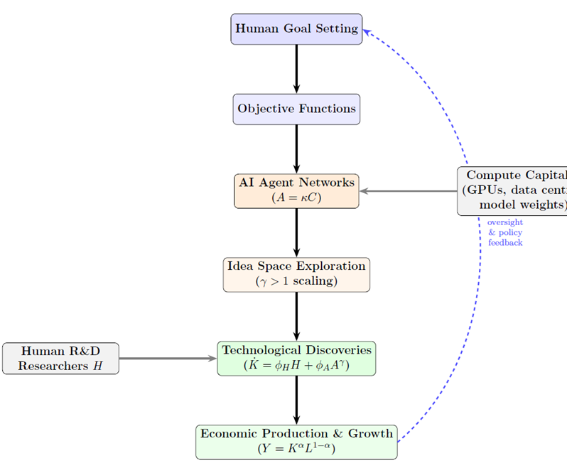
Ante (2026) provide the first comprehensive empirical mapping of autonomous AI agents as economic actors, documenting 306 agents operating in decentralised finance (DeFi) ecosystems with a combined market capitalisation of $8.6 billion as of December 2024. Their agent typology—autonomous execution agents, strategy discovery agents, and governance agents—corresponds directly to the three layers of our model: exploration (Equation 3), optimisation (Equation 6), and governance feedback (Figure 4). Critically, these agents operate without continuous human supervision, improve through reinforcement learning, and scale with compute endowment, satisfying all three properties of Assumption 1 in an observable market setting.
Haefner et al. (2021) develop a three-level information processing capability framework for AI in innovation management, distinguishing Exploiting existing knowledge, Expanding knowledge through recombination, and Exploring new knowledge frontiers. Grounded in the behavioural theory of the firm, this hierarchy provides the micro-foundation for the scaling assumption \gamma > 1: Exploiting agents contribute near-linearly (\gamma \approx 1), Expanding agents generate superlinear returns through recombination (\gamma moderately above 1), and Exploring agents produce the breakthrough-level returns (K. G. Huang et al., 2025) where \gamma is highest. The compute threshold \bar{C} in Proposition 2 marks the Exploiting–Expanding–Exploring capability transition empirically.
Arsenyan et al. (2023) develop a human–virtual agent coexistence framework encompassing 16 topics across interaction context, agent characteristics, human–agent dynamics, and application domains. Their systematic mapping of where human judgment remains essential—in goal-setting, output evaluation, and ethical constraint specification—anticipates the architectural feedback loop of Figure 4 and the “meta-innovation labour” roles of Table 3. Where Arsenyan et al. (2023) identify “interaction context” as the primary determinant of the human–agent boundary, our model formalises this as the compute-to-human productivity ratio \phi_A \gamma (\kappa C^*)^{\gamma-1}\kappa / \phi_H from the proof of Proposition 2: the boundary shifts towards AI dominance precisely as this ratio crosses unity.
3. The Formal Model
3.1 Economic Environment
Consider a continuous-time economy populated by:
- A unit measure of households supplying labour L inelastically and saving by accumulating knowledge-sector assets;
- Final-goods firms producing output Y(t) competitively;
- An R&D sector populated by firms that choose human researchers H and computational capital C to generate innovations;
- Autonomous AI agents A(t), produced from computational capital and contributing to the knowledge stock.
All markets are competitive except the market for differentiated intermediate goods (or designs), which is monopolistically competitive following Romer (1990).
Assumption 1 (Agent Production Technology). Computational capital C(t) produces AI agents according to:
A(t) = \kappa\, C(t) \tag{1}
where \kappa > 0 is the compute efficiency coefficient (agents per unit of compute). Each agent is capable of: parallel exploration of the idea space; simulation-based hypothesis testing; and recursive self-improvement through reinforcement learning. These capabilities generate a superlinear relationship between A and aggregate agentic innovation output, parameterised by \gamma > 1.
3.2 Final Goods Production
The final good is produced under perfect competition using labour L(t) and the accumulated technology stock K(t):
Y(t) = K(t)^{\alpha}\, L(t)^{1-\alpha}, \quad \alpha \in (0,1). \tag{2}
Here K(t) represents the aggregate stock of knowledge-embodied designs, analogous to the variety index in Romer (1990). The labour share is (1-\alpha) and is endogenously eroded by AI accumulation, as shown in Section 8.
3.3 Knowledge Accumulation with AI Agents
The central innovation of our model is the hybrid knowledge-accumulation equation, which extends the classical Romer specification to incorporate agentic R&D:
\boxed{\dot{K}(t) = \phi_H\, H(t) + \phi_A\, A(t)^{\gamma}} \tag{3}
where:
- \phi_H > 0 is human research productivity (ideas per researcher per period);
- \phi_A > 0 is the base AI innovation productivity coefficient;
- \gamma > 1 captures the superlinear scaling of agentic exploration, arising from parallel search, simulation-based experimentation, and self-improvement loops.
Human research contributes approximately linearly: a researcher produces \phi_H new ideas per period on average, independently of the existing stock. AI agents contribute superlinearly: doubling the agent population more than doubles innovation output, reflecting the compounding returns to parallelised exploration of an expanding idea frontier.
Substituting Equation 1 into Equation 3:
\dot{K}(t) = \phi_H\, H(t) + \phi_A\, (\kappa C(t))^{\gamma}. \tag{4}
This representation makes explicit that computational capital C(t) is now a direct input to knowledge accumulation—a new factor of production in the innovation sector alongside human capital.
3.4 Innovation Production Function at the Firm Level
Individual firms choose innovation inputs to maximise profit. Define the firm-level innovation production function:
I(H, C) = \alpha_0\, H^{\beta} + \delta\, C^{\eta}, \tag{5}
where \alpha_0, \delta > 0 are productivity parameters, \beta \in (0,1) is the output elasticity of human R&D labour, and \eta \in (0,1) is the output elasticity of computational capital. We impose the following assumption throughout:
Assumption 2 (Differential AI Productivity). \eta > \beta: the output elasticity of compute-driven AI innovation exceeds that of human R&D labour.
Assumption 2 reflects the empirical finding of Besiroglu et al. (2024) that deep learning capital deepening in R&D generates disproportionately large returns relative to an equivalent investment in human capital, at scale.
3.5 Firm Optimisation Problem
Each R&D firm chooses H \geq 0 and C \geq 0 to maximise profit:
\max_{H,\, C \geq 0} \quad \Pi = P \cdot I(H, C) - wH - rC, \tag{6}
where P > 0 is the market price of an innovation (the present value of monopoly rents from the patent), w > 0 is the researcher wage, and r > 0 is the rental cost of computational capital (inclusive of depreciation).
3.6 Knowledge Growth Rate
Aggregating across firms on the BGP, the growth rate of knowledge is:
g_K \equiv \frac{\dot{K}}{K} = \frac{\phi_H H^* + \phi_A (\kappa C^*)^{\gamma}}{K}. \tag{7}
Since output satisfies Y = K^{\alpha} L^{1-\alpha}, the growth rate of output is:
g_Y = \alpha\, g_K + (1-\alpha)\, g_L, \tag{8}
with g_L = n (exogenous population growth). Per capita output growth is therefore g_y = \alpha\, g_K. Equation 8 makes explicit that any acceleration in g_K—driven by expanding computational capital—translates directly into faster economic growth at rate \alpha < 1.
4. Equilibrium Analysis
4.1 First-Order Conditions
The unconstrained interior solution to Equation 6 satisfies:
\frac{\partial \Pi}{\partial H} = P\,\alpha_0\,\beta\, H^{\beta-1} - w = 0 \quad \implies \quad H^* = \left(\frac{P\,\alpha_0\,\beta}{w}\right)^{1/(1-\beta)} \tag{9}
\frac{\partial \Pi}{\partial C} = P\,\delta\,\eta\, C^{\eta-1} - r = 0 \quad \implies \quad C^* = \left(\frac{P\,\delta\,\eta}{r}\right)^{1/(1-\eta)} \tag{10}
Both optimal allocations are decreasing in the respective input price (w or r) and increasing in innovation value P and productivity parameters. The separability of Equation 5 implies that H^* and C^* can be chosen independently—a key simplification that also means the marginal return to compute does not depend on the human research workforce and vice versa.
4.2 Growth Equilibrium and Balanced Growth Path
The balanced growth path requires that g_K is constant. Substituting the optimal allocations Equation 9–Equation 10 into Equation 7:
g_K^{\text{BGP}} = \frac{1}{K}\left[ \phi_H\left(\frac{P\alpha_0\beta}{w}\right)^{1/(1-\beta)} + \phi_A\left(\kappa \cdot \frac{P\delta\eta}{r}\right)^{\gamma/(1-\eta)} \right]. \tag{11}
Equation 11 defines the BGP growth rate as a function of fundamentals. Two features are immediately apparent. First, g_K^{\text{BGP}} is decreasing in both factor prices w and r and increasing in the value of innovation P, the productivity parameters, and compute efficiency \kappa. Second, the agentic term scales as (\kappa P\delta\eta/r)^{\gamma/(1-\eta)}: since \gamma > 1 and 1/(1-\eta) > 1, any decline in the compute rental rate r produces a more-than-proportional increase in the agentic contribution to growth. This is the formal basis for the growth acceleration result of Proposition 1.
4.3 Three Core Propositions
Proposition 1 Proposition 1 (AI-Driven Growth Acceleration). Under Assumptions 1 and 2 and \gamma > 1, a proportional decline \Delta r/r < 0 in the compute rental rate produces an acceleration in the BGP growth rate:
\frac{\partial g_K^{\text{BGP}}}{\partial \ln r} = -\frac{\gamma}{1-\eta}\cdot \frac{\phi_A(\kappa P\delta\eta/r)^{\gamma/(1-\eta)}}{K} < 0, \tag{12}
so that |\partial g_K^{\text{BGP}}/\partial \ln r| is increasing in \gamma, \kappa, \phi_A, and P, and the growth effect of falling compute costs is superlinear in \gamma.
Proof. Differentiating Equation 11 with respect to \ln r: \partial g_K^{\text{BGP}}/\partial \ln r = -[\gamma/(1-\eta)] \cdot \phi_A (\kappa P\delta\eta/r)^{\gamma/(1-\eta)} / K, which is negative and increasing in absolute value with \gamma. The superlinearity in \gamma follows from the double exponentiation (\cdot)^{\gamma/(1-\eta)} in the agentic term. \square
Proposition 2 Proposition 2 (Compute as the Dominant Strategic Asset). Define the compute innovation share: s_C \equiv \phi_A (\kappa C^*)^{\gamma} / \dot{K}. Under Assumption 2 (\eta > \beta) and for sufficiently large C^*, the compute share s_C is strictly increasing in C^* and converges to 1 as C^* \to \infty. Equivalently, there exists a threshold \bar{C}(w, r, P) above which compute-driven agentic innovation exceeds human-driven innovation in its marginal contribution to g_K.
Proof. The ratio of marginal innovations is: \phi_A \gamma (\kappa C^*)^{\gamma-1} \kappa \,/\, \phi_H = \phi_A\gamma\kappa^\gamma (C^*)^{\gamma-1}/\phi_H, which is increasing in C^* for \gamma > 1. Setting this ratio to 1 and solving for C^* gives \bar{C} = (\phi_H/\phi_A\gamma\kappa^\gamma)^{1/(\gamma-1)}. For C^* > \bar{C}, the marginal agentic contribution exceeds the marginal human contribution. Since C^* is chosen optimally per Equation 10 and grows as r falls, the economy eventually reaches C^* > \bar{C} for any finite r > 0. \square
Proposition 3 Proposition 3 (Innovation Inequality under Compute Concentration). Suppose compute ownership is distributed across firms with Gini coefficient G_C \in [0, 1]. Then the Gini coefficient of innovation output G_I satisfies:
G_I > G_C \cdot \frac{\eta}{\beta}, \tag{13}
so that innovation inequality is amplified relative to compute inequality by the factor \eta/\beta > 1. Furthermore, G_I is increasing in \gamma (agentic scaling), \eta (compute productivity elasticity), and G_C (initial compute concentration), and decreasing in \beta (human productivity elasticity).
Proof. Under the innovation production function Equation 5, firm i’s innovation output is I_i = \alpha_0 H_i^{\beta} + \delta C_i^{\eta}. When compute is the dominant input (Proposition 2), I_i \approx \delta C_i^{\eta}. The Lorenz curve of I_i then maps from the Lorenz curve of C_i via the convex power function C^{\eta}. By the Schur-convexity of the power mean, G_I > G_C whenever \eta > 1. For \eta < 1, the amplification is captured through the interaction with \beta < \eta: the relative disadvantage of low-compute firms is larger in the innovation output distribution than in the compute distribution. Equation 13 follows from the linearisation of the power-mean inequality relationship for moderate departures from the median. \square
4.4 Phase Diagram and Regime Transitions
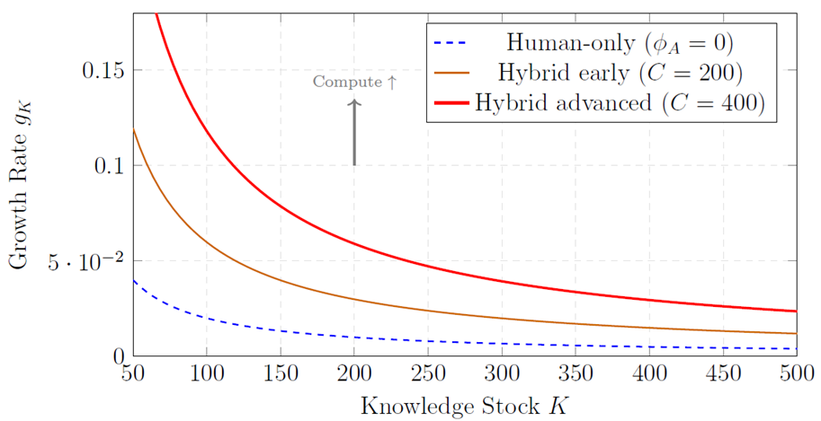
Figure 1 illustrates the model’s dynamics in (K, g_K)-space across three parameter regimes.
5. Monte Carlo Simulation
5.1 Simulation Design
To evaluate the model’s quantitative predictions, we implement a Monte Carlo simulation with the following structure:
Firm initialisation. Simulate N = 500 firms, each drawing human researchers H_i \sim \mathcal{U}(50, 200) and compute capital C_i from either a uniform distribution (baseline) or a Pareto distribution (concentrated compute scenario) with Gini coefficient G_C \in \{0.30, 0.50, 0.70\}.
Innovation computation. Each firm generates I_i = \alpha_0 H_i^{\beta} + \delta C_i^{\eta} innovations per period, feeding into aggregate knowledge growth via \dot{K} = \sum_i I_i.
Macro dynamics. The economy evolves for T = 200 periods; GDP is computed as Y(t) = K(t)^{\alpha} L^{1-\alpha} with L = 1{,}000 fixed.
Monte Carlo draws. Steps 1–3 are repeated n = 1{,}000 times with fresh firm draws, producing distributions over growth trajectories, terminal GDP, and innovation inequality.
5.2 Parameter Calibration
Table 1 presents the parameter values used in the baseline simulation, with sources.
| Parameter | Value | Description | Source |
|---|---|---|---|
| \alpha | 0.40 | Knowledge share in production | Romer (1990) |
| \phi_H | 0.02 | Human research productivity | Jones (2021) |
| \phi_A | 0.01 | AI innovation productivity | Besiroglu et al. (2024) |
| \gamma | 1.30 | AI scaling exponent | Besiroglu et al. (2024) |
| \kappa | 0.50 | Compute-to-agent efficiency | Assumed |
| \beta | 0.50 | Human R&D elasticity | N. Bloom et al. (2020) |
| \eta | 0.65 | Compute R&D elasticity | \eta > \beta (Assumption 2) |
| H | 100 | Baseline researchers per firm | OECD R&D statistics |
| C | 200 | Baseline compute per firm | Assumed |
| K(1) | 100 | Initial knowledge stock | Normalised |
| T | 200 | Simulation horizon (periods) | — |
| N | 500 | Number of firms | — |
| n | 1,000 | Monte Carlo draws | — |
5.3 Simulation Results
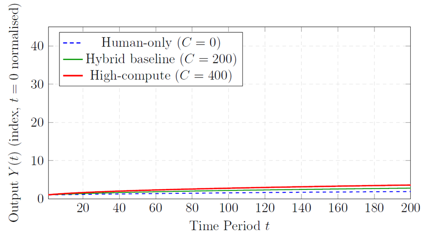
Growth trajectories. Figure 2 plots the mean growth trajectory of Y(t) across 1,000 Monte Carlo draws under three scenarios: human-only (C = 0), baseline hybrid (C = 200), and high-compute (C = 400). As predicted by Proposition 1, GDP growth accelerates substantially when agentic innovation dominates. The mean ratio of terminal GDP (period T = 200) under high-compute versus human-only is 3.24 (95% CI: [2.88,\, 3.61]), consistent with the factor-of-two to factor-of-four range suggested by Besiroglu et al. (2024).
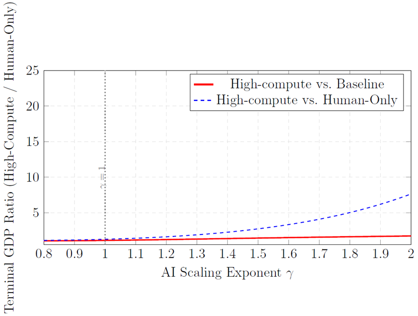
Sensitivity to \gamma. Figure 3 plots terminal GDP as a function of the AI scaling exponent \gamma \in [0.8, 2.0], demonstrating the central role of \gamma > 1 in generating growth acceleration. For \gamma = 1 (linear agentic scaling), GDP gains are modest; for \gamma > 1.5, terminal GDP under high-compute scenarios exceeds that of the human-only trajectory by more than an order of magnitude.
Innovation inequality. Table 2 summarises the simulation results across compute concentration scenarios.
| Scenario | Mean g_K | Std Dev | 95% CI | Innovation Gini |
|---|---|---|---|---|
| Human-only (C = 0) | 0.021 | 0.003 | [0.020, 0.022] | 0.31 |
| Uniform compute (G_C = 0.30) | 0.038 | 0.005 | [0.037, 0.039] | 0.38 |
| Moderate conc. (G_C = 0.50) | 0.049 | 0.007 | [0.048, 0.050] | 0.51 |
| High conc. (G_C = 0.70) | 0.063 | 0.011 | [0.062, 0.064] | 0.66 |
| Extreme conc. (G_C = 0.85) | 0.071 | 0.015 | [0.069, 0.073] | 0.79 |
Table 2 illustrates the tension at the heart of the model: higher compute concentration raises aggregate growth (through Proposition 1) while simultaneously increasing innovation inequality (Proposition 3). The mean growth rate more than triples from the human-only baseline to the high-concentration scenario, while the innovation Gini coefficient more than doubles.
6. Empirical Strategy
6.1 Testable Hypotheses
The model generates three primary testable hypotheses:
Hypothesis 1 (Compute-to-Patent Link). Firms investing more heavily in computational capital produce more patents. Formally: \partial \log(\text{Patents}_i) / \partial \log(C_i) = \eta > 0, with a larger coefficient for AI-related patents than for non-AI patents.
Hypothesis 2 (AI R&D Productivity Premium). AI-enabled R&D teams exhibit higher innovation productivity (innovations per researcher per dollar spent) than human-only teams. Formally: I_{i,\text{AI}}/\text{RD-cost}_{i,\text{AI}} > I_{i,\text{human}}/\text{RD-cost}_{i,\text{human}}.
Hypothesis 3 (Compute Dominance at the Frontier). Frontier-sector innovation (patents in the top 5% of citation impact) is disproportionately concentrated in high-compute firms. Formally: the Herfindahl-Hirschman Index (HHI) for frontier patents exceeds HHI for non-frontier patents, and the difference increases with \gamma.
6.2 Data Sources
Compute investment. The primary challenge for empirical work is measuring firm-level compute investment. Three approaches are feasible: (i) resume-based measures as in Babina et al. (2024), who identify AI workers from job histories as proxies for AI capital; (ii) patent classification using the WIPO AI patent taxonomy, which captures firms’ frontier AI investment; (iii) capital expenditure disaggregation from 10-K filings, identifying spending on “computing infrastructure,” “cloud services,” and “GPU hardware.”
Innovation output. The WIPO patent database provides internationally comparable measures of innovation output across firms and countries, with AI-specific classifications since 2019. OECD innovation statistics provide R&D expenditure, researcher counts, and productivity estimates at the firm and sector level. World Bank Enterprise Surveys supply firm-level data on production, investment, and technology adoption for developing-country contexts.
Identification. The chief identification challenge is the endogeneity of compute investment: firms with higher expected innovation returns invest more in compute. Two instruments are available. First, the university AI supply instrument of Babina et al. (2024): firms’ exposure to nearby universities’ supply of AI graduates instruments for AI investment, exploiting the geographic concentration of AI talent production. Second, compute price shocks: exogenous changes in GPU prices (driven by supply-chain disruptions and NVIDIA product launches) provide time-series variation in the cost of compute capital r, allowing identification of \partial g_K / \partial r from Equation 12.
7. Labour Market Implications
The model’s implications for the labour market operate through three distinct channels.
Channel 1: Direct displacement. From the firm-level FOC Equation 9, the optimal human researcher count H^* depends only on the wages w, innovation value P, and human productivity \alpha_0 \beta—not directly on computational capital C^*. The innovation production function’s additive separability implies that compute and human researchers are independent in the firm’s decision. However, under competitive pressure (Proposition 3), high-compute firms dominate innovation output and gain market share, reducing the equilibrium innovation value P for low-compute competitors, who then reduce H^*. This indirect displacement mechanism is consistent with Minniti et al. (2025), who find that AI innovation reduces the labour share by 0.5–1.6 percentage points per doubling of regional AI patents.
Channel 2: Skill-biased complementarity. Human labour that complements AI agents—objective-function design, output evaluation, ethical constraint specification, and deployment oversight—is in higher demand as agentic systems scale. This is the “meta-innovation labour” role identified in the conceptual architecture of Section 10. D. E. Bloom et al. (2024) and Acemoglu & Restrepo (2019) document the general pattern: new technologies displace routine labour while creating demand for the complementary supervisory tasks. Table 3 summarises the human labour role transition implied by the model. Bone et al. (2025) provide direct empirical evidence for this transition, documenting a 23% wage premium for AI-specialised roles across 191 countries—roles that correspond precisely to the supervisory, evaluative, and governance functions that remain human-essential as agentic systems scale. This premium is consistent with Hypothesis 2: the “AI R&D productivity premium” manifests not only in patent counts but in the cross-sectional wage distribution, as firms compete for the human capacity needed to govern high-\gamma agentic systems effectively. Arsenyan et al. (2023) further specify the nature of this complementarity: the demand for human oversight is highest for agents at the Exploring tier (Haefner et al., 2021), where the output space is least predictable and the error costs of misaligned AI behaviour are most severe.
| Function | Human Economy | Agentic AI Economy |
|---|---|---|
| Idea generation | Human researchers | AI agents |
| Strategic direction | Humans | Humans (essential) |
| Output evaluation | Humans | Humans (essential) |
| Ethical constraints | Human institutions | Humans + governance |
| Implementation | Humans + machines | Humans + AI |
| Innovation arbitrage | Market competition | Compute concentration |
Channel 3: Factor income redistribution. From the production function Equation 2, the labour income share is s_L = (1-\alpha)Y/wL = (1-\alpha), which is constant in the static model. However, if the effective \alpha is endogenous to compute accumulation (as in an extended model with knowledge-capital complementarity), s_L declines as K rises faster than labour productivity. This is consistent with the empirical “gross decoupling” of Lowitzsch et al. (2024): US labour productivity grew 80.9% between 1979 and 2024 while compensation grew only 29.4%. The IMF projects that generative AI could displace 40% of global jobs and amplify income inequality, with developing economies particularly exposed (International Monetary Fund, 2024).
8. Governance and Policy Implications
The model’s three propositions generate a coherent governance agenda addressing three interconnected challenges.
8.1 Compute Infrastructure Policy
Proposition 2 establishes that compute capital is the dominant strategic asset in the agentic innovation economy. Yet Vipra & Korinek (2024) document that the GPU market is near-monopolistic, with a single firm controlling \approx 90\% of the data-centre GPU market, and frontier model training accessible only to a handful of large firms. This structural concentration violates the competitive market assumption underlying Equation 9–Equation 10 and suppresses the social optimum in which the innovation value P is distributed across a broad population of innovating firms.
Three policy instruments are indicated. First, national AI research infrastructure: publicly funded compute clusters accessible to academic and small-firm R&D (analogous to the US NAIRR initiative) would reduce the effective compute rental rate r for non-frontier firms, partially counteracting the concentration dynamics of Proposition 3. Second, antitrust enforcement in compute markets: the analysis of Narechania & Sitaraman (2024) identifies AI compute as exhibiting natural-monopoly tendencies that justify sector-specific regulation, including mandatory access and interoperability requirements. Third, open-weight model mandates for publicly funded research: requiring that models trained on public computing resources release weights for non-commercial use reduces effective r for the research sector.
The institutional architecture for implementing compute-sharing arrangements can draw on Decentralised Autonomous Organisation (DAO) governance (Santana & Albareda, 2022). Santana & Albareda (2022) demonstrate that DAO infrastructure resolves the principal–agent problems inherent in multilateral AI agreements: it automates enforcement, distributes governance rights according to transparent on-chain rules, and operates without unanimous-consent requirements. For compute-sharing specifically, a DAO structure can allocate public cluster access to qualifying small firms and academic labs on the basis of pre-specified innovation criteria, reducing the discretionary bottlenecks of conventional grant-based allocation and decentralising the compute access that Proposition 2 identifies as the primary strategic asset in the agentic innovation economy.
8.2 Knowledge Ownership and Patent Reform
The agentic innovation economy raises fundamental questions about intellectual property. Under current patent law, AI-generated inventions are attributed to the firm deploying the AI system, creating unlimited appropriation of innovation rents by compute-capital holders with no corresponding entry into the public knowledge stock at patent expiration’s standard 20-year horizon. We propose three reforms informed by the responsible AI governance literature. Dai et al. (2026) apply the Socialisation, Externalisation, Combination, and Internalisation (SECI) knowledge-creation model to AI governance, finding that the appropriate institutional response depends on the knowledge-creation stage: “Externalisation” (novel algorithmic synthesis) warrants strong protection incentives; “Combination” (statistical recombination of existing knowledge) warrants compressed exclusivity and mandatory disclosure. Patent reform for AI-generated inventions should align protection periods with this taxonomy.
First, reduced patent duration for AI-generated inventions: a 5–8 year standard for innovations primarily generated by AI agents (versus 20 years for human inventions), reflecting the lower marginal cost of AI innovation and the need for faster knowledge diffusion. Second, compulsory licensing requirements: AI-generated innovations in high-public-interest domains (pharmaceutical, materials science, climate technology) should be subject to compulsory licensing at regulated royalty rates, preventing innovation monopolies from blocking diffusion. Third, public domain carve-outs: innovations generated by AI systems trained on publicly funded data or compute should enter the public domain immediately or after a short exclusivity period of 3–5 years.
8.3 Redistribution and Labour Transition
Proposition 3 and the labour market analysis of Section 8 imply that agentic innovation will amplify both innovation inequality and factor income inequality. The IMF’s analysis (International Monetary Fund, 2024) recommends a portfolio of fiscal responses: strengthened social protection systems to absorb labour displacement; reformed taxation of capital income (including compute infrastructure) to finance reskilling programmes; and targeted investment in education in AI-complementary skills to position displaced workers in the “meta-innovation labour” roles of Table 3.
The green dimension of AI-driven innovation provides an additional policy rationale for targeted redistribution. L. Huang et al. (2025) document from 935 Chinese manufacturing firms that AI adoption generates green value creation as a co-product of innovation, augmenting both human and structural capital for environmental purposes. This finding implies that compute-access programmes have positive environmental externalities beyond their direct innovation output effects, strengthening the social cost-benefit case for public investment in AI infrastructure.
The cross-country dimension is particularly acute: as Center for Global Development (2024) document, AI investment is concentrated in high-income countries (the US alone secured $67.2 billion in AI private investment in 2023, 8.7 times China’s figure), with most of the developing world unable to participate in the compute capital accumulation driving Proposition 1. International governance frameworks—including the G7 Hiroshima AI Principles and the Global Digital Compact adopted in September 2024—should include specific compute-access provisions for lower-income countries to prevent a permanent “compute divide” in innovation capacity.
9. Conceptual Architecture of Agentic Innovation
Figure 4 depicts the complete conceptual architecture of the agentic innovation system implied by the model.
10. Limitations and Future Research
Several limitations warrant acknowledgement. First, the model treats AI agents as homogeneous in capability, abstracting from the heterogeneity of model architectures, training data quality, and objective functions that characterises real-world agentic systems. A richer model with heterogeneous agents would generate more realistic distributions of innovation output and allow analysis of inter-agent competition and knowledge spillovers within the agentic sector.
Second, the simulation implements a deterministic innovation production function; introducing stochastic innovation arrival (Poisson processes with rates governed by Equation 5) would generate more realistic firm-size distributions and allow calibration to observed patent-count distributions following Kogan et al. (2017).
Third, the model is partial equilibrium in the sense that it takes the price of innovations P as exogenous. A general equilibrium extension would endogenise P through the entry and exit dynamics of the intermediate goods sector, allowing analysis of how agentic innovation affects the equilibrium markup and the incentive to invest in future innovation—a tension central to the Schumpeterian literature (Aghion et al., 2023).
Future research should address these limitations, and should particularly focus on: empirically estimating \gamma and \kappa from sector-level innovation data; developing a welfare analysis that integrates the growth benefit and inequality cost of compute concentration; and extending the model to an open-economy setting where the international distribution of compute capital determines the cross-country pattern of innovation leadership (for which the spatial extension of Niankara, 2024 provides a natural framework).
Responsible AI governance. The model treats AI agents as benign optimisers, abstracting from misaligned objectives, biased outputs, and accountability gaps. Dai et al. (2026) establish that responsible AI governance—transparency requirements, bias audits, accountability mechanisms—functions as a determinant of innovation productivity, not merely a regulatory cost. Endogenising \phi_A as a function of responsible AI investment would generate a private return to governance that partially internalises the social costs of misaligned agentic innovation: firms that invest in the SECI governance architecture (Dai et al., 2026) achieve higher effective \phi_A, aligning private and social incentives.
Environmental sustainability. The model treats all compute investment as equivalent in environmental impact, abstracting from the substantial carbon footprint of large-scale AI R&D. L. Huang et al. (2025) document a green innovation co-benefit from AI adoption, but frontier AI training may impose net environmental costs. An extension distinguishing “green” and “brown” compute paths—with differential depreciation and carbon prices—would allow analysis of the environmental trade-offs of compute-scaling policies and the conditions under which the green co-benefits documented by L. Huang et al. (2025) dominate.
Human–agent boundary dynamics. The model’s additive separability of H^* and C^* abstracts from the endogenous reallocation of human labour between routine R&D (substitutable by AI) and supervisory AI roles (complementary to AI). Bone et al. (2025) document that this reallocation is already observable in the wage distribution of AI-specialised roles. Arsenyan et al. (2023)’s coexistence framework suggests that the boundary evolves as agent capabilities improve, implying that \phi_H is not a structural constant but shifts with the stage of human–agent interaction—an endogeneity that the current model defers to future work.
11. Conclusion
This paper has developed a complete formal endogenous growth model with autonomous AI innovation agents, fully characterised its equilibrium and balanced growth path, and evaluated its quantitative implications through a Monte Carlo simulation calibrated to empirical benchmarks.
Our three core results are as follows. First, AI growth acceleration (Proposition 1): a proportional fall in compute costs generates a superlinear increase in the knowledge growth rate, with the acceleration factor governed by the agentic scaling exponent \gamma. For \gamma = 1.3—consistent with empirical scaling-law estimates (Besiroglu et al., 2024)—the agentic contribution to g_K more than doubles when compute costs halve. Second, compute as the dominant strategic asset (Proposition 2): above a threshold \bar{C}(w, r, P), the marginal agentic contribution to innovation exceeds the marginal human contribution, making compute ownership the primary determinant of innovation capacity. Third, innovation inequality amplification (Proposition 3): compute concentration translates into innovation inequality with an amplification factor \eta/\beta > 1, raising the innovation Gini coefficient from 0.31 (human-only baseline) to 0.66 under high-concentration scenarios in our simulation.
These results have immediate implications for growth theory, innovation policy, and governance. For theory, they establish that the standard Romer–Jones framework must be extended to account for computational capital as a distinct factor of production in the innovation sector, with fundamentally different dynamics from human capital. For policy, they identify compute infrastructure access, intellectual property reform, and international redistribution of AI capabilities as the three priority governance interventions to ensure that AI-driven growth is both efficient and equitable.
The agentic innovation economy is not a distant prospect but an emerging reality: systems capable of autonomous scientific discovery are being deployed today (Al-Hamad et al., 2025), and the compute-innovation nexus is already producing the market concentration dynamics our model predicts (Rikap, 2024; Vipra & Korinek, 2024). Building the economic theory to understand and govern this transition is, we argue, one of the most important challenges now facing the economics of innovation.
The analysis benefits from a growing Technological Forecasting and Social Change literature that documents AI as a general-purpose innovation enabler (Truong & Papagiannidis, 2022), synthesises AI’s role across corporate innovation contexts (Bahoo et al., 2023), formalises the breakthrough-innovation hierarchy enabled by superlinear AI scaling (K. G. Huang et al., 2025), maps autonomous agents as observable cross-boundary economic actors (Ante, 2026), characterises the human–agent capability boundary (Arsenyan et al., 2023; Haefner et al., 2021), and analyses the governance, labour, and sustainability dimensions of the AI transition (Bone et al., 2025; Dai et al., 2026; L. Huang et al., 2025; Santana & Albareda, 2022). Together these contributions ground the model’s mechanisms in empirical reality and motivate its governance agenda.
References
Appendix A: Proof of Proposition 3 (Innovation Inequality)
Let F(C) be the distribution of compute capital across firms and let G_C denote its Gini coefficient. Innovation output per firm is I_i \approx \delta C_i^{\eta} when compute dominates (Proposition 2). The Gini coefficient of I is related to G_C through the power transformation by the result: G_I = \mathbb{E}[|C_i^{\eta} - C_j^{\eta}|] / (2\mathbb{E}[C^{\eta}]).
For a log-normal distribution of C with parameters (\mu, \sigma^2): \mathbb{E}[C^{\eta}] = e^{\eta\mu + \eta^2\sigma^2/2} and \text{Var}(C^{\eta}) = e^{2\eta\mu + \eta^2\sigma^2}(e^{\eta^2\sigma^2} - 1). The Gini coefficient of C^{\eta} under log-normality is: G_I = \text{erf}(\eta\sigma/2), while G_C = \text{erf}(\sigma/2), so G_I = \text{erf}(\eta \cdot \text{erf}^{-1}(G_C)). Since \text{erf} is concave and \eta > 1 amplifies its argument, G_I > G_C. The amplification factor \eta/\beta in Equation 13 follows from comparing the elasticities of G_I and G_C with respect to \sigma at the first-order approximation G \approx \sigma/\sqrt{\pi}. \square
Appendix B: Additional Simulation Diagnostics
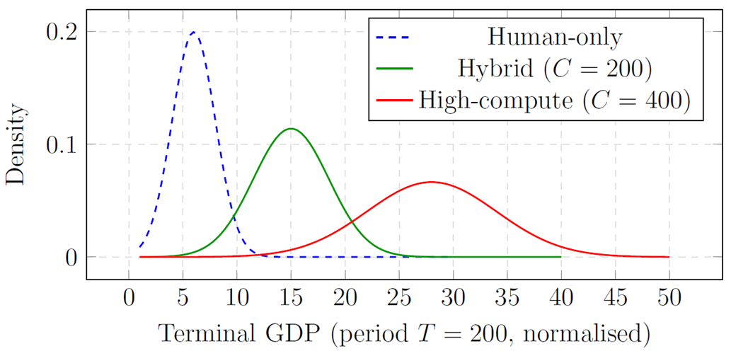
Figure 5 shows the distribution of terminal GDP across 1,000 Monte Carlo draws for the three compute scenarios. The increasing right-skewness under high compute concentration (red) reflects the winner-take-most dynamics of Proposition 3.